Anyone managing a project eventually confronts the same fundamental question: how do I measure schedule performance in a way that gives me reliable, actionable information? The answer lies not in a single metric or a quick glance at a Gantt chart, but in a disciplined set of activities grouped under the Control Schedule process. Project managers draw on performance reviews, variance analysis, and, where applicable, earned value management or critical chain methods to assess how the project is tracking against the plan. The purpose is to detect deviations early, understand their causes, and decide whether a response is necessary before small delays cascade into missed deadlines. Measuring schedule performance means looking beyond simple date comparisons and examining work progress, resource usage, buffer consumption, and the behavior of the project’s network logic.
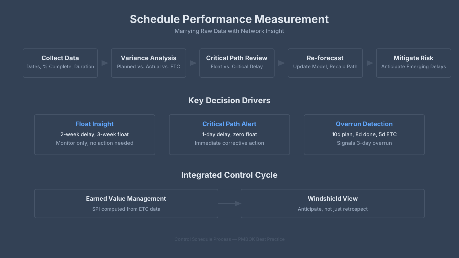
Schedule Performance Measurement: Key Points Summary
| Key Concept | Summary |
|---|---|
| Control Schedule | Schedule performance is proactively managed by detecting variances early and applying corrective measures to prevent minor slippages from cascading into critical delays. |
| Performance Reviews | Performance reviews serve as the primary diagnostic for schedule health, systematically contrasting actual progress against the baseline to inform targeted adjustments. |
| Actual Dates | Actual start and finish dates supply unfiltered timeline data, instantly highlighting early-stage delays that warrant root cause investigation. |
| Percent Complete | Percent complete indicators require careful interpretation; a package near completion may still be behind schedule if it has surpassed its target finish date while burning extra budget. |
| Variance Analysis | Variance analysis quantifies the extent and severity of schedule deviations, then drives deeper investigation into underlying causes during structured status reviews. |
| Critical Path | Any delay on the critical path immediately forecasts a later project completion date; tasks with generous float can absorb limited slippage without jeopardizing the overall deadline. |
| Review Frequency | Review cadences are calibrated to project dynamics, from daily stand-ups in fast-paced Agile environments to milestone-based evaluations in multi-year infrastructure programs, ensuring timely interventions. |
| Duration Estimates | Task owners project remaining effort, and when that estimate plus elapsed effort surpasses the original duration, the resulting variance points to root causes such as scope expansion, resource constraints, or underestimated complexity. |
How Performance Reviews and Variance Analysis Measure Schedule Performance
The core mechanism for assessing schedule health is the performance review, which uses actual project data to compare what has been accomplished against the baseline plan. Actual start and finish dates give the raw timeline facts: a task planned to start on the 5th of the month that actually commenced on the 12th already has a seven-day lag. Percent complete figures tell a more nuanced story; a work package reported as 60 percent complete might look healthy until you realize it has consumed 80 percent of its budget and is already two weeks past its planned finish. Remaining duration for work in progress adds a forward-looking component, often estimated by the team members doing the work, which transforms a historical review into a what-will-it-take-to-finish analysis. When these three data streams are pulled together during regular status meetings, variance analysis measures schedule performance by evaluating the magnitude of departure from the schedule baseline and probing its causes.
A purely mechanical comparison of dates can be misleading if not filtered through an understanding of project logic. A task that slips by several weeks on a path with abundant total float may not threaten the overall end date, while a one-day delay on the critical path directly pushes out the finish. Performance reviews, therefore, integrate network analysis into schedule measurement. In the PMBOK Guide, this falls under the Monitor and Control Process Group, and the Control Schedule process explicitly calls for comparing actual results to the schedule baseline and then analyzing variances. The review is not a one-time event but a recurring discipline, with frequency linked to the project’s rhythm—daily stand-ups in Agile contexts, weekly in traditional iterative phases, or milestone-driven in long-term construction programs.
Comparing Actual Dates, Percent Complete, and Remaining Duration
The simplest dimension of schedule performance compares actual start and finish dates against planned dates. Yet seasoned project managers know that a completed task does not always signal smooth progress if it finished late and caused downstream rework. Percent complete becomes indispensable for in-flight activities, but it requires careful interpretation. A developer might report “90 percent done” for three consecutive weeks, and suddenly the remaining 10 percent balloons into new unforeseen tasks. The real value emerges when percent complete is combined with remaining duration. Task owners estimate how many more working days are needed; if that number plus the elapsed time exceeds the original duration by a significant margin, schedule variance is evident, and the root cause may be scope creep, underestimated complexity, or resource unavailability.
Imagine a design activity with a two-week baseline. After five working days, the team reports 30 percent complete and estimates another 10 days remaining. The total duration would stretch to 15 working days, a 50 percent overrun. The performance review surface this and then variance analysis digs into the why: perhaps the client’s feedback cycles are slower than expected, or the designer is also supporting another project. Without the remaining duration data, the percent complete figure alone would not trigger an alert because 30 percent after five days in a ten-day task seems roughly on track. The combination of metrics makes the discrepancy visible and prompts a deeper inquiry.
Earned Value Management: SV and SPI to Measure Schedule Performance
When organizations use earned value management, schedule variance (SV) and the schedule performance index (SPI) provide a numeric, trendable view of how the project is performing against its planned schedule. SV is the difference between earned value (the planned cost for the work actually performed) and the planned value (the planned cost for the work that should have been done at this point). A negative SV means the project has accomplished less than planned, a positive value signals ahead-of-schedule performance. SPI, the ratio of earned value to planned value, normalizes this so that an SPI of 1.0 means exactly on schedule, below 1.0 indicates a lag, and above 1.0 points to an advance.
These earned value metrics measure schedule performance in monetary terms, which can cause confusion if treated as a direct calendar measure. SPI, for example, declines linearly with a schedule slip only if the remaining work’s value is proportional to time, which may not hold. A more robust practice is to use SPI in conjunction with a time-based index or a to-complete schedule performance index to forecast the finish date. In large government or defence programmes, EVM is mandatory, and the calculated SV and SPI for work breakdown structure components, work packages, and control accounts become the formal record of schedule performance. The SPI trend over several reporting periods reveals whether the project is recovering, stable, or deteriorating—information far more powerful than a single snapshot.
Critical Chain Buffer Monitoring for Schedule Performance Assessment
In projects managed with the critical chain method, the primary instrument for schedule performance assessment is buffer management. The project buffer protects the delivery date, and feeding buffers protect the critical chain. Instead of tracking task-level start and finish dates against a detailed baseline, the team monitors how much of the buffer has been consumed compared to how much of the chain has been completed. If the project has progressed 40 percent through the critical chain but has already consumed 70 percent of the buffer, the buffer is being used up faster than work is being finished, which signals that corrective action is urgently needed. Conversely, if buffer consumption stays proportionally lower than chain progress, the schedule is healthy.
This approach shifts the conversation from blaming individual task delays to assessing systemic flow. A task that takes longer than its aggressive estimate simply eats into the buffer that was designed to absorb such variability. The real alarm bell rings when buffer penetration crosses a predetermined trigger threshold. Many practitioners use a fever chart—a green, yellow, red graphic that plots buffer consumption against chain completion—to communicate schedule status instantly. This method of schedule performance assessment avoids the micro-management of date-driven reporting and focuses management attention on the big-picture trajectory of the project end date.
Key Insights on Schedule Measurement
- Performance reviews compare actuals to baseline
- Performance reviews serve as the primary control for schedule integrity, directly comparing actual accomplishments against the baseline to identify deviations early and enable proactive corrective action.
- Percent complete reveals budget consumption
- A work package reported as 60 percent complete often conceals serious trouble when it has already consumed 80 percent of its budget and is overdue against its planned finish date, signalling scope expansion or persistent productivity gaps.
- Remaining duration adds forward-looking insight
- By estimating the remaining workdays, teams generate a forward-looking metric; when the total of elapsed and remaining duration exceeds the original plan, schedule variance becomes evident, typically driven by scope creep, underestimated complexity, or resource bottlenecks.
- Variance analysis evaluates departure magnitude
- In routine status meetings, variance analysis quantifies the scale of deviations from the schedule baseline and triggers root-cause investigation, consistent with the Control Schedule process within the PMBOK Monitor and Control Process Group.
- Critical path determines delay impact
- A delay of several weeks on a path carrying abundant total float may not threaten the project finish date, whereas a single day’s slip on the critical path immediately postpones completion.
Determining When a Schedule Variation Requires Corrective Action
Not every schedule variation deserves a response. Measuring schedule performance is only half the picture; the other half is applying judgment to decide whether a deviation will materially affect the project’s objectives. A major delay on a non-critical path activity might look alarming on a task-level report, but if the activity has abundant total float, the project finish date remains unaffected. Total float analysis is critical for corrective action decisions because it reveals how much leeway exists before a delay transforms from an inconvenience into a critical threat.
The project manager must triage variances. For a delay on a near-critical activity—one with only a few days of total float—the situation may demand immediate attention even though technically it is not yet on the critical path. Near-critical paths represent a risk of criticality that can materialize suddenly if the task consumes its remaining float. Variance analysis therefore evaluates not just the size of the delay but its location in the network diagram. An assessment that ignores float and focuses solely on absolute time drift will misallocate management attention, perhaps spending resources to recover a non-critical task while the true schedule risk lies unnoticed on a parallel path.
Distinguishing Critical Path Delays from Non-Critical Path Variances
The critical path method defines the longest sequence of activities that determines the project’s earliest possible finish. Any delay on this path is a direct, day-for-day extension of the project deadline. So when measuring schedule performance, a one-week slip on a critical task is far more significant than a three-week slip on a task with ten days of total float. Yet the common trap is to react to the sheer size of a variance rather than its systemic impact. In a rapidly unfolding project, a subcontractor might report a three-week delay on a non-critical equipment installation. The schedule measurement system will flag it as a variance, but the float analysis will show that the overall completion date is unchanged. The wise project manager acknowledges the variance, monitors it, but does not immediately reallocate resources from critical tasks to solve a non-critical problem.
Communication with stakeholders often centres on this distinction. Senior leaders who see a large delay in a status report may demand action regardless of the float analysis. The project manager’s role includes translating the measurement data into a risk-informed narrative that distinguishes real threats from variances that the project can absorb. The same logic applies when using schedule performance metrics like SPI; SPI might be below 1.0 because of delays on non-critical work that will not affect the finish date, yet the number alone might trigger an unjustified escalation.
Using Total Float Variance to Evaluate Project Time Performance
Total float variance is an essential but underappreciated indicator of project schedule health. It measures the change in total float for activities or paths over successive update cycles. A narrowing of total float on a near-critical path signals emerging schedule pressure that demands attention before it becomes critical. If a path that originally had eight days of total float now shows only two days after a reporting period, something has consumed that buffer quietly without necessarily causing an overt schedule variance on the path’s activities. This kind of trend analysis surfaces schedule performance issues that pure date comparisons miss.
Monitoring float variance across the entire network often reveals systematic problems such as resource bottlenecks, undisciplined change control, or optimistic reporting that erodes slack gradually. Many scheduling tools can generate float variance reports automatically, but their value depends on the project manager’s diligence in reviewing them. When float vanishes on multiple paths simultaneously, the project is approaching a point where a single additional disruption could push the finish date out significantly. The float variance, interpreted alongside SV and SPI data, gives a more complete picture of schedule performance measurement than any single technique alone.
Documenting and Communicating Schedule Performance Measurements
All the analysis in the world counts for nothing if the resulting work performance measurements are not documented and communicated clearly to stakeholders. The outputs of the Control Schedule process include schedule variance and schedule performance index values calculated for work breakdown structure components, work packages, and control accounts. Documenting schedule performance measurements ensures that decisions about corrective or preventive actions are based on a traceable, factual record. When a steering committee asks why a milestone was missed, the project manager can point to the SV and SPI trends and the float analysis that signalled the drift weeks earlier.
These measurements become part of the project’s formal records and feed into performance reports and stakeholder communications. The format matters: raw EVM numbers can confuse an audience not familiar with earned value, so narratives and visual representations like S-curves, buffer charts, or milestone trend charts often supplement the data. The documented performance measures also form the baseline for any change requests related to the schedule. If a schedule rebaseline is proposed, the historical SV, SPI, and float variances justify the need and scope of the change.
How Work Performance Measurements Are Distributed to Stakeholders
The specific calculated values—SV and SPI for WBS components, work packages, and control accounts—must be packaged appropriately for different stakeholder groups. A project sponsor may only need a high-level SPI trend and a summary of the top schedule risks. A functional manager providing resources might need the SV data at the control account level to understand which work packages are lagging. The project team itself benefits from seeing the buffer consumption status or the float trend so that they can self-correct before management intervention. Distribution timing also aligns with the project’s governance rhythm, whether that means monthly portfolio reviews, bi-weekly sprint reviews, or quarterly program board meetings.
In Agile environments, the equivalent concept might be the burndown or burnup chart, which communicates how much work remains against the iteration timeline. While the terminology differs, the principle of making schedule performance visible is identical. The Scrum Master or Agile coach uses the sprint burndown during daily stand-ups to signal whether the team is on track to meet the sprint goal. This form of transparent schedule performance measurement supports the Agile value of empiricism—inspecting and adapting based on real data. The documentation then lives in the team’s toolset, accessible to anyone who needs to see the trend.
From a program management perspective, the aggregated SV and SPI data across multiple projects becomes a portfolio schedule health indicator. Program managers look for systemic patterns: are all projects consuming float faster than expected? Is SPI consistently below 1.0 across a group of initiatives? Such patterns might point to organizational bottlenecks like a shared design team that is overcommitted, and the program-level schedule performance measurement triggers corrective action at a higher system level. The documentation chain from work package to program provides a seamless audit trail that supports governance and accountability, reinforcing the purpose of measuring schedule performance as a management discipline rather than a compliance exercise.
The final piece of the communication puzzle is ensuring that the measurement data leads to decisions. A status report that merely reports a declining SPI without a recommended action is only half done. The Control Schedule process expects that variance analysis will include determining the cause and degree of variation relative to the schedule baseline so that a decision can be made about whether corrective or preventive action is needed. When the project manager presents the measurements, they must also offer options: should we fast-track certain tasks, add resources, accept the delay, or adjust the scope? The work performance data becomes the foundation for these choices, and clear documentation makes it possible to justify the chosen course later.
Key Takeaways on Performance Communication
- Documentation establishes traceable accountability
- Documenting schedule variance and SPI values creates a factual, traceable record that supports corrective decisions and equips project managers to present steering committees with the early warning signals underlying missed milestones.
- Tailored visuals improve stakeholder clarity
- Narratives and visual tools such as S-curves and buffer charts translate complex earned value data into clear, accessible insights for stakeholders unfamiliar with EVM.
- Distribution aligns with audience and cadence
- Functional managers receive schedule variance data at the control account level to identify lagging work packages, while project teams monitor buffer consumption and float trends, all delivered on a cadence that matches the governance review rhythm.