When a project manager needs to cut through the noise of status reports and gut-feel assessments, earned value management project performance measurement provides a disciplined, numbers-based alternative. It is not just a reporting exercise. Earned value management, or EVM, fuses scope, schedule, and cost into a single analytical framework, letting you see whether your project is truly on track, drifting, or heading for a crisis long before subjective impressions catch up. The approach builds on a simple but powerful idea: by assigning a monetary value to each planned activity, you can compare what you planned to spend, what you actually spent, and what you physically accomplished, all in the same unit of measure. This allows for early warning signals that other methods miss entirely. Yet despite its conceptual elegance, many practitioners only scratch the surface of what EVM can reveal. The real insight emerges when you move beyond the formulas and start interpreting the patterns that variance and efficiency data create over time. Understanding those patterns requires a clear grasp of the baseline that makes all subsequent analysis possible.
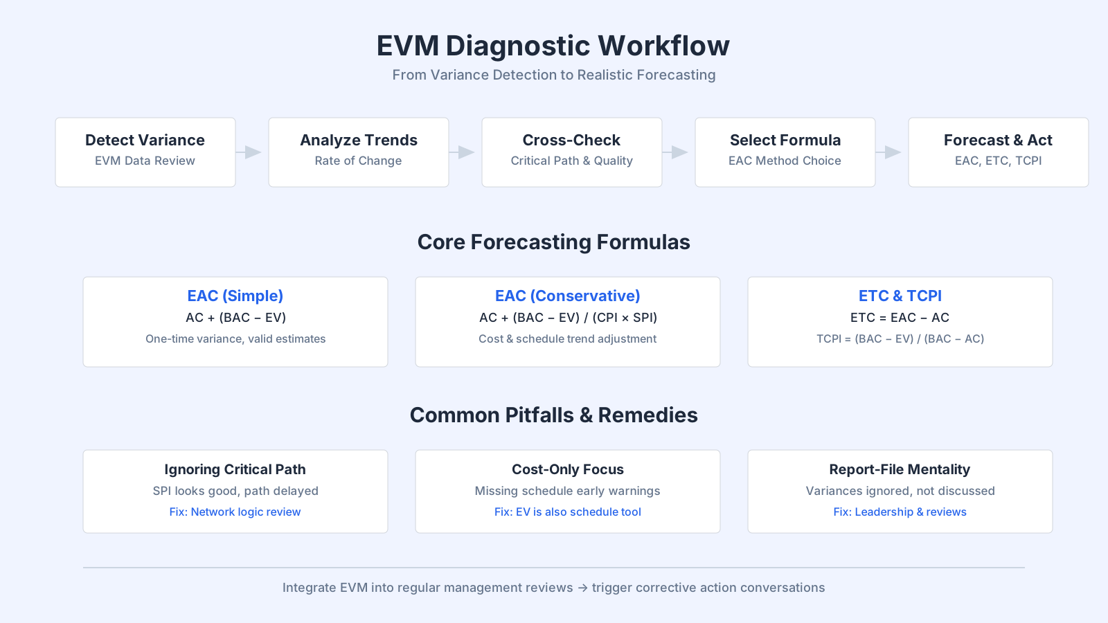
Earned Value Management at a Glance
| Key Concept | Summary |
|---|---|
| EVM | Earned value management integrates scope, schedule, and cost into a single analytical framework, revealing genuine project performance before subjective assessments can obscure reality. |
| Core Idea | By assigning a monetary equivalent to each planned activity, EVM enables a direct comparison of planned work value, actual expenditures, and physical accomplishment within a unified financial language. |
| Baseline | Every credible EVM analysis depends on a performance measurement baseline that fuses scope, schedule, and cost into one authoritative reference point, serving as the objective yardstick for deviation detection. |
| PMBOK Context | The baseline, an output of the Planning Process Group, relies on a mature Work Breakdown Structure crafted during scope definition, anchoring execution to the agreed scope from the outset. |
| Scope Creep | When scope expands without formal baseline updates, performance is measured against an obsolete plan, rendering all calculated variances hollow and decision-making unreliable. |
| Living Document | On dynamic projects, the baseline must be treated as a living document, evolving through formally approved change requests to stay aligned with shifting realities and preserve analytical validity. |
| Planned Value | For a control account, Planned Value begins at zero, accumulates as scheduled work unfolds according to the master schedule, and ultimately equals the full budget at completion, forming the essential benchmark for schedule performance measurement. |
| PV Pitfall | Modeling Planned Value as a purely linear distribution ignores actual resource profiles and workload intensity, often producing misleading early schedule variances that mask true progress and delay corrective action. |
Understanding the Earned Value Management Baseline
Every meaningful EVM analysis rests on a carefully constructed performance measurement baseline that integrates the project scope, schedule, and cost parameters into a single reference point. This baseline is not simply a budget spreadsheet or a Gantt chart. It represents the approved plan for what work will be performed, when it will be performed, and how much it is authorized to cost. In PMBOK terms, the baseline falls squarely within the Planning Process Group, under the Project Cost Management and Project Schedule Management knowledge areas, and it draws heavily on the Work Breakdown Structure created during scope definition. Without a properly decomposed WBS that breaks the project into control accounts and work packages, the baseline becomes too coarse to support reliable EVM calculations.
The baseline assigns a time-phased budget value to every discrete work package. This aggregated sum, known as the Budget at Completion or BAC, is the total planned value from which all subsequent metrics flow. For the baseline to serve its purpose, it must be maintained through formal change control. If scope creeps in without a corresponding adjustment to the baseline, the EVM numbers start telling a lie: actual performance gets compared against an outdated plan, and variances become meaningless. Practitioners often underestimate how much discipline this demands. In fast-moving projects where scope churn is a fact of life, the baseline can quickly become irrelevant unless the project manager treats it as a living document that evolves through documented, approved changes.
A common misconception is that the baseline is only for large, waterfall-style projects. While EVM originated in defense and construction programs with rigid phases, the concept of a performance measurement baseline is perfectly adaptable to iterative development environments. The key is to baseline smaller chunks of work, perhaps at the iteration or release level, and to accept that the BAC may shift as the backlog evolves. What remains constant is the need to have a defined reference point against which you measure progress. Without that, you are merely tracking spending, not performance.
Planned Value: The Authorized Budget Distributed Over Time
Planned value, or PV, is the foundation stone of the baseline. It represents the cumulative budget that was scheduled to be spent on an activity or work package up to a given point in time. Think of it as the time-phased budget baseline that answers the question: as of today, how much did we intend to spend if everything happened exactly according to plan? For a given control account, PV starts at zero and grows as scheduled activities are expected to be executed, eventually reaching the full BAC when the work is complete. Setting PV accurately requires more than simply dividing the total budget by the number of months. You must reflect the actual timing of resource usage, procurement commitments, and work effort. S-shaped curves are typical because project spending tends to ramp up gradually, reach a peak, and then taper off.
One frequent mistake is to construct PV as a purely linear distribution, ignoring the resource loading profiles that real schedules demand. If you have a heavy testing phase at the midpoint of a software project, for example, the PV curve should reflect that bulge. Failing to do so will cause the EVM analysis to show a false schedule variance later: you might appear behind schedule in early weeks when, in reality, your plan never intended to spend much during that period. The shape of the PV curve matters as much as its total value. A project manager who understands that shape can also use it to have a more nuanced conversation with stakeholders about why a negative schedule variance in a particular month does not necessarily signal disaster.
Earned Value: The Budgeted Value of Completed Work
Earned value, or EV, is the metric that often creates the greatest confusion for newcomers to EVM, yet it is the linchpin of the entire system. EV represents the budgeted cost of the work that has actually been performed up to the status date. Notice the critical distinction: it is not what you spent, nor what you planned to spend; it is what you have accomplished, valued at the original budget rates. If a work package has a total PV of $10,000 and you have completed exactly half of that work, the EV for that package is $5,000, regardless of how much money you actually spent achieving that progress. This decouples physical progress from financial expenditure and allows the true cost and schedule performance to be measured independently.
Determining EV objectively is where many projects stumble. For some work packages, physical completion can be assessed with reasonable accuracy through concrete acceptance criteria or milestones. In knowledge work, such as software development or research, completion percentages can be notoriously subjective. The common practice of a developer claiming that a feature is "90% done" for weeks on end is the enemy of reliable EVM. To combat this, many organizations adopt discrete measurement techniques like the 50/50 rule, where 50% of the budget is earned when the activity starts and the remaining 50% when it finishes, or the 0/100 rule, where nothing is earned until complete. These methods introduce a conservative bias that prevents over-optimistic EV inflation and keeps the data honest.
Another nuance that experienced project managers watch for is the ceiling that EV naturally imposes: earned value for any work package can never exceed its planned value. Once you have completed the authorized scope, you stop earning value against that budget, even if unforeseen additional work was required. Any extra effort is either covered by a management reserve drawdown or constitutes an unplanned overrun. This constraint is not a flaw; it is a deliberate design that highlights scope creep and inefficiency. When EV plateaus while AC continues to rise, you have a powerful visual signal that something is consuming resources beyond the original plan.
Actual Cost: The Real Financial Outlay
Actual cost, or AC, is the most straightforward of the three core EVM data points but is frequently undercut by inconsistent accounting practices. It is the total cost incurred for the work performed during the measurement period, recorded in the same way that the budget was allocated to planned value. If PV and EV are expressed in terms of direct labor hours, materials, and overhead, then AC must capture those same categories faithfully. Discrepancies in how costs are accumulated, for example, when labor is tracked from timesheets but subcontractor invoices lag by a month, can skew the entire analysis. The golden rule is alignment: the cost definition used for AC must mirror the definition used for PV and EV. If you planned for fully burdened labor rates in the baseline, using unburdened rates for AC will make cost performance look artificially favorable.
Getting AC right is as much an organizational discipline as a project management task. The project manager often relies on finance systems that were not designed for EVM reporting cadences. Monthly accounting closes can create a one-month lag in cost data, making real-time monitoring difficult. In such environments, some teams maintain shadow tracking of committed costs and accruals to get a nearer-to-real-time picture. This extra effort is worth it only if the project's size and risk profile justify the overhead, but for programs where EVM is a contractual requirement, such adjustments become part of the daily rhythm. The moment you lose confidence in your AC numbers, the CV and CPI metrics that follow become untrustworthy, and you are back to navigating by instinct.
Essential Takeaways on EVM Baselines
- Integrated reference point
- The Performance Measurement Baseline integrates scope, schedule, and cost into a single unified benchmark, providing the sole reference for all earned value calculations.
- WBS decomposition is essential
- A thoroughly decomposed Work Breakdown Structure, organized into control accounts and detailed work packages, is fundamental for producing accurate and reliable earned value metrics.
- BAC anchors all metrics
- The Budget at Completion aggregates the total planned value; it serves as the baseline from which all EVM metrics and variance analyses originate.
- Guard against scope creep
- Uncontrolled scope creep, not accompanied by formal baseline revisions, undermines EVM integrity; treat the baseline as a living document updated only through authorized change control.
- PV follows resource profiles
- Planned Value must mirror actual resource loading profiles, incrementing from zero to the full BAC in a pattern that avoids unrealistic linear distribution over time.
Calculating Schedule and Cost Variances Effectively
Once the three foundational numbers are in place, the real diagnostic work begins by calculating schedule variance and cost variance at both the control account level and the overall project level. These variances are startlingly simple: SV equals EV minus PV, and CV equals EV minus AC. Yet the simplicity conceals the depth of interpretation they invite. A variance is not just a red flag; it is a prompt to ask why the plan and reality diverged. A large negative SV could stem from a delayed approval, a resource shortage, an underestimated activity, or simply a poorly distributed PV curve. The variance itself only tells you there is a gap; the analysis of root causes requires going deeper into the WBS to isolate the offending work packages.
One of the most useful properties of schedule variance is that it automatically converges to zero at project completion, assuming the project does finish. When all planned work is done, EV equals PV equals BAC, and SV becomes zero by definition. This means that a positive SV in the middle of the project is not a permanent gain; it indicates that you earned more value earlier than planned, but it does not guarantee that you will finish early. Conversely, a negative SV signals that you are behind today, but if the pace of execution increases, the variance can shrink. The transient nature of SV is why relying on it alone for schedule forecasting can be misleading; performance indices are needed to project forward, but we will come to those later.
Interpreting Schedule Variance in Real-World Projects
Let’s examine what SV looks like in practice without naming any specific company. Imagine a mid-sized construction project where the foundation work was planned to be complete by the end of month three, with a corresponding PV of $200,000. At that review point, the actual physical completion of the foundation corresponds to an EV of only $150,000. The SV is minus $50,000. The easy interpretation is that the project is behind schedule by roughly a quarter of the foundation budget. The more refined interpretation is that the cause might be weather delays, not poor productivity, which means the schedule variance might be recovered once conditions improve. If the project manager had simply reported "we are behind," without the EVM numbers, stakeholders might not appreciate that the cost side remains healthy because AC might also be $150,000, yielding no cost overrun despite the schedule slip.
The ability to separate schedule impact from cost impact in a single data point is what gives EVM its diagnostic power. When both SV and CV are negative, the project is in trouble on two fronts, and management attention needs to be ramped up. When SV is negative but CV is positive or near zero, the issue is likely one of sequencing or resource allocation rather than financial waste. This distinction changes the type of corrective action you take, from accelerating specific activities to reassigning resources, rather than simply demanding across-the-board budget cuts.
Analyzing Cost Variance and Its Permanence
Cost variance behaves very differently from schedule variance, and this is a point that many project managers miss until they have been burned by it. Unlike SV, a negative CV does not automatically zero out at project completion. If you spend more to accomplish a given amount of work, that overrun is locked in; there is no magical recovery mechanism unless you can later perform remaining work for less than its budgeted cost. A negative CV today is, in most cases, a permanent overrun on the work already completed. This characteristic makes CV a particularly sobering metric. When you see a cumulative CV of negative $30,000 at the halfway point, you are not just $30,000 over budget; you are on a trajectory that could compound if the same inefficiencies persist.
The psychology of cost variance reporting can also be tricky. When a team sees a significant negative CV early in the project, there is often a temptation to try to "earn back" the loss by seeking efficiencies in the remaining work. While this is sometimes possible through value engineering or simplified approaches, the EVM framework assumes that future work will be performed at the planned productivity unless there is evidence to the contrary. Underestimating the drag of a negative CV leads to unrealistic Estimates at Completion. A healthy practice is to treat any negative CV as a lesson that requires a root-cause analysis: were the original estimates simply too low, or did unplanned rework consume resources? The answer determines whether you need to rebaseline or simply adjust procurement strategies.
Using Trend Analysis and S-Curves for Performance Forecasting
Beyond point-in-time variances, the real predictive value of EVM emerges when you apply trend analysis with S-curves to visualize performance trajectories. An S-curve displays the cumulative values of PV, EV, and AC over time, creating a picture that even non-financial stakeholders can grasp quickly. The PV curve typically follows that characteristic S shape, starting slow, accelerating, then flattening. The EV curve should ideally hug the PV curve, and the AC curve should, in a perfect world, sit right on top of EV. Divergence between these curves is the visual story of project health. When the AC curve climbs above the EV curve, you have a cost overrun; when EV lags behind PV, you have a schedule delay. The separation grows or narrows as performance changes, and the eye can detect accelerating problems far faster than scanning a table of numbers.
Trend analysis layers on top of the S-curve by examining the rate of change of these divergences. A project that has a stable, negative cost variance is one thing; a project where the CV is getting worse each month is another matter entirely. The slope of the cumulative CV line tells you whether the overrun is growing, steady, or being brought under control. A manager seeing a consistently worsening trend might intervene before the cost overrun becomes catastrophic. Conversely, a narrowing gap between EV and PV indicates that schedule recovery actions are working. Trend analysis transforms EVM from a reactive reporting tool into a forward-looking decision support system.
Visualizing Performance with Cumulative and Periodic Charts
One mistake that orgs make is to only examine cumulative S-curves. Cumulative data smooths out the short-term tempo of work and can hide problems that are only visible when you look at weekly or monthly snapshots. If a team had a terrible month but the cumulative curve still looks acceptable, management might miss a significant deterioration in recent productivity. Supplementing the cumulative view with periodic charts, tables that break down EV, PV, and AC by individual reporting period, can reveal that a trend reversal has just begun. The raw numbers for a single period might show EV below PV for the first time in six months, an early signal that cumulative variance might soon turn negative if not addressed.
These periodic views also help separate seasonal or planned variations from genuine drift. A maintenance shutdown month will naturally show low EV; that is baked into the PV curve. The periodic chart shows that both PV and EV dropped in parallel, so no variance arises. The cumulative chart alone might cause a stakeholder to panic because the total EV growth slowed. Layering the two perspectives gives a more nuanced understanding, and experienced project managers learn to toggle between them depending on the audience and the specific question at hand.
From Trends to Forecasted Completion Costs
The S-curve does more than display the past; it allows you to project a likely end point for the actual cost line. This Estimate at Completion, or EAC, is one of the most requested outputs of an EVM system. The simplest projection assumes that future cost performance will follow the same efficiency as the cumulative CPI to date. That forecasted AC curve might shoot far above the BAC line on the graph, providing a stark warning. More sophisticated approaches create a range of EACs using different assumptions: one where the remaining work is performed at the originally planned rate, and another where the current inefficiency is expected to persist. By expressing these as a fan of possible endpoints, you present decision-makers with a risk-informed view rather than a single, potentially misleading number.
S-Curve Forecasting Key Insights
- S-curves visualize performance trajectories
- By plotting cumulative planned value, earned value, and actual cost on a single timeline, the S-curve transforms complex data into an intuitive visual that enables rapid comprehension across all stakeholder levels.
- PV curve follows characteristic pattern
- The planned value curve naturally mirrors an S-shaped growth pattern, with gradual ramp-up during early phases, acceleration through peak execution, and a final flattening as deliverables near completion.
- Trends outpace number tables
- Shifts in the gap between curves signal trouble much earlier than raw numbers ever could, allowing stakeholders to spot accelerating variances at a glance rather than by laboriously comparing columnar data.
- Cumulative data masks short-term issues
- Because cumulative curves absorb short-term fluctuations, pairing the S-curve with period-specific charts that isolate EV, PV, and AC per reporting interval uncovers nascent trend reversals that would otherwise remain hidden.
- Multiple EAC assumptions forecast futures
- Advanced forecasting generates a spectrum of estimate-at-completion values by varying assumptions, for example projecting that remaining work will proceed at the original budgeted rate versus assuming that current cost efficiency trends continue unabated.
Efficiency Metrics: SPI and CPI as Performance Gauges
Variances tell you the magnitude of deviation in absolute terms, but Schedule Performance Index and Cost Performance Index normalize that deviation into efficiency ratios that can be compared across work packages, projects, and portfolios. SPI is EV divided by PV, and CPI is EV divided by AC. An index of 1.0 means performance exactly matches the plan. Values below 1.0 flag inefficiency, while values above 1.0 indicate favorable performance. Because these are unitless ratios, they allow comparisons that would be impossible with raw dollar variances. A $10,000 schedule variance on a $100,000 package feels different from the same variance on a $2 million package, but an SPI of 0.90 communicates the same 10% inefficiency regardless of scale.
The CPI, in particular, has taken on the role of the project's financial pulse. In many industries, a CPI below 0.90 is a threshold that triggers mandatory corrective action boards or even stop-work reviews. The reason is that cumulative CPI tends to stabilize after the first 20% of the project, after which it becomes a reliable predictor of final cost performance. This stabilization occurs because early variances set the tempo for how the team works with the budget; radical changes in efficiency are rare unless management intervenes forcefully. So the CPI you see at the one-third mark is likely, though not guaranteed, to be close to the final CPI when the project closes. That empirical observation gives CPI outsized weight in program reviews.
The Schedule Performance Index and Its Limitations
SPI is conceptually clean but carries a subtle limitation that becomes critical near the end of a project. Since SPI uses PV in the denominator, and PV eventually hits the BAC ceiling and stops growing, SPI can give misleading signals in the final stages. If a project is nearing completion, EV catches up with PV, and SPI gravitates toward 1.0 even if the project is late because the PV no longer increases to reflect the remaining schedule. To address this, some practitioners switch to a time-based SPI called SPI(t), which measures schedule performance against the planned duration rather than budgeted cost. This advanced metric requires a separate schedule baseline but provides a more stable indicator for forecasting completion dates.
Where SPI really shines is during the execution phase, when the bulk of PV is still ahead. At that point, an SPI consistently below 0.95 signals that the project is slipping and that the original delivery date is at risk. It prompts a schedule risk analysis that may lead to crashing or fast-tracking activities. The power of SPI comes from its ability to make schedule delays tangible in cost terms, which often resonates more with finance-oriented stakeholders than a percentage-complete chart ever could.
The Cost Performance Index as a Warning System
CPI is often called the most critical EVM metric, and for good reason. It is the ratio that most directly translates into a financial forecast. A CPI of 0.80 means that for every dollar of budgeted value being earned, $1.25 is being spent. Extrapolated over the remaining BAC, that paints a grim picture. Unlike schedule delays that can sometimes be absorbed by overlapping phases, cost overruns have a direct impact on the project business case. The project manager who monitors CPI weekly can detect negative shifts while they are still small. A CPI that drops from 1.02 to 0.98 over two reporting periods may not seem alarming, but if the trend continues, a major overrun is brewing. By the time CPI hits 0.80, the project has already sustained significant damage.
One practice that sharpens CPI analysis is to segment it by work package or cost account. An overall project CPI of 0.95 might mask a subcontracted workstream running at 0.70 while the in-house team is at 1.10. Drilling down reveals that the overall project is being dragged down by a single troubled area. Targeted management attention can then be directed to renegotiating the subcontract or providing technical support, rather than cutting resources across the board. This granularity moves the conversation from "we are over budget" to "this specific scope is over budget, and here is what we are doing about it." That is a world apart.
Integrating EVM into Ongoing Project Monitoring and Control
The full utility of earned value management is realized only when it becomes embedded in routine project monitoring and not treated as a monthly report that gets filed and forgotten. Integrating EVM into project monitoring means setting a consistent cadence, typically weekly or aligned with your sprint review cycle, for collecting actual progress data, recalculating EV and AC, and analyzing fresh variances. This rhythm aligns with the Monitoring and Controlling Process Group in PMBOK, specifically the Control Costs and Control Schedule processes, which feed directly into integrated change control. The data generated by EVM becomes the factual backbone for decisions about corrective actions, resource reallocation, and baseline changes, replacing opinion with analysis.
Successful integration also requires that the EVM data be presented in a format appropriate for each stakeholder group. The project team needs detailed control account reports to manage their own work. The sponsor needs a dashboard that highlights cumulative CPI, SPI, and a forecast EAC against the BAC, with trend arrows. What no one needs is a raw dump of formulas. The translation from EVM metrics to management actions is where many initiatives fail. A project manager who says "our CV is negative $15,000" loses the room; one who says "we've spent $15,000 more than we earned last month, and that overrun is concentrated in testing rework, which we are now addressing by adding automated checks" commands confidence.
Aligning EVM with PMBOK and Agile Practices
From a PMBOK perspective, EVM is the bridge that connects the Cost Management and Schedule Management knowledge areas with the data-driven analysis demanded by the Monitor and Control process group. The technique provides objective inputs for variance analysis, a tool explicitly listed under Control Costs. It directly supports the Work Performance Data to Work Performance Information conversion, as raw EV, PV, and AC numbers are transformed into variances, indices, and forecasts. PRINCE2 environments, while using a different terminology, have an equivalent focus on tolerances and stage boundaries where EVM data can serve as the factual underpinning for exception plans and highlight reports. In Agile contexts, traditional EVM might seem out of place, but adaptations are common. Many organizations calculate EV based on story points accepted in an iteration, with PV derived from the planned velocity and a cost per point derived from team burn rate. The indexes then become useful for forecasting release dates and costs, though they must be interpreted more loosely given the variable scope nature of Agile.
One thing to watch for is the temptation to impose EVM on every project regardless of its complexity. EVM was designed for large, definable-scope efforts where the overhead of rigorous tracking is justified by the financial risk. On a small, short-duration project, the administrative burden can outweigh the benefits, and a simplified burn-down chart may suffice. Knowing when to scale back EVM applications to only key performance indicators is a sign of a mature project management culture. The BVOP methodology, for example, emphasizes value delivery and waste reduction, and would caution against implementing EVM in a way that overburdens the team. In BVOP, tracking could focus on Business Value Points delivered per iteration, with EVM-like metrics applied only to significant workstreams, not every tiny task, to avoid the process damage that comes from excessive oversight.
Common Pitfalls in Applying Earned Value Management
Even rigorously calculated EVM data can lead to poor decisions if certain pitfalls are not recognized. One of the most pervasive is the "schedule variance as cost" trap. Because SV is expressed in monetary units, project sponsors sometimes mistakenly treat a positive SV as money in the bank. It is not; it is just an apples-to-apples comparison that allows schedule to be measured against plan. You cannot spend schedule variance. Another trap is using EVM numbers in isolation without considering external factors that affect performance. A perfect CPI might result from cutting corners on quality, something that EVM alone would not reveal until defects cascade. Therefore, EVM should always be paired with quality metrics and technical performance measures.
A deeper organizational pitfall is the blame culture that EVM can inadvertently foster. When a CPI drops below 1.0, the knee-jerk reaction is to find the person responsible. In reality, root causes are often systemic: poor initial estimates, shifting requirements, or resource bottlenecks that no single person controls. A mature organization uses EVM data to learn and adjust its estimating processes, not to punish individuals. The difference in outcomes is vast. Finally, there is the pitfall of neglecting to maintain the baseline. If the baseline is not updated for approved changes, the EVM data will show phantom variances that provoke useless discussions while the real execution problems go unaddressed. The baseline is a model, and like any model, it requires upkeep.
Making EVM a Decision-Making Tool, Not a Report Card
The ultimate goal of measuring project performance with EVM is to empower better, faster decisions. When a project manager sits down with the cumulative S-curve and the CPI/SPI trend charts, the question should never be "what is our status?" because the charts already show that. The question should be "what are we going to do about it?" If CPI is trending down, is the response a change request to increase the budget, a reprogramming of scope, or an aggressive efficiency drive? The EVM data defines the size of the problem, but management judgment determines the solution. Projects that succeed in embedding EVM as a decision tool often establish trigger points, pre-agreed actions that kick in when certain thresholds are breached, so that decisions are not endlessly debated. A CPI below 0.85 might automatically trigger a reserve draw request and a mandatory rebaselining review. That depersonalizes the response and speeds up the governance cycle.
When EVM is used this way, it shifts the entire project dynamic from reactive firefighting to proactive performance management. You start to see patterns before they become crises. You can have honest conversations with stakeholders about trade-offs while there is still time to adjust. The numbers do not solve problems, but they make the problems impossible to ignore and the solutions testable against a clear baseline. That is, in the end, what measuring project performance is really about.
Key Takeaways on EVM Integration
- Consistent EVM data cadence
- Embedding EVM into a steady weekly or sprint‑based rhythm for capturing progress, updating earned value and actual cost, and interpreting emerging variances unlocks its full value.
- EVM as an evidence-based decision tool
- EVM data provides the factual foundation for corrective actions, resource rebalancing, and baseline adjustments; project managers who articulate the root cause and corrective path for an overrun inspire significantly more confidence than those who merely report the unfavorable variance.
- Framework alignment for EVM adoption
- Across methodologies, EVM aligns with PMBOK’s Control Costs and Control Schedule processes, reinforces PRINCE2’s tolerance management and exception planning at stage boundaries, and within BVOP concentrates on Business Value Points exclusively for the most impactful workstreams.