Activity duration estimating sits at the core of every project schedule, yet the process is rarely straightforward. Anyone who has tried to pin down exactly how long a task will take knows that a single number rarely captures reality. Traffic patterns shift, a key team member gets pulled into another assignment, a vendor deliverable arrives a day late, and suddenly that crisp estimate is off by a significant margin. Three-point estimating addresses this by acknowledging uncertainty head-on, replacing the fiction of a single deterministic number with a range of possibilities and a calculated weighted average that serves as the expected duration. The technique traces its roots to the Program Evaluation and Review Technique, better known as PERT, and remains one of the most reliable ways to produce accurate activity duration estimates for complex or uncertain work.
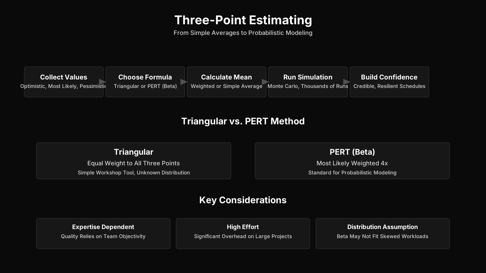
Summary of Three-Point Estimating for Activity Durations
| Key Concept | Summary |
|---|---|
| Three-point estimating | Three-point estimating replaces fixed duration estimates with a range of optimistic, most likely, and pessimistic values. A weighted average then yields the expected duration, explicitly capturing uncertainty rather than presenting an artificially precise single number. |
| PERT origins | The technique originated with the Program Evaluation and Review Technique (PERT), developed during the U.S. Navy's Polaris missile program to model schedule uncertainty across large-scale, interdependent defense systems. |
| Single-point problem | A single-point estimate fosters a deceptive sense of precision, failing to disclose whether it reflects an optimistic scenario, a conservatively padded figure, or the mean of a broad probability distribution. |
| Optimistic estimate | The optimistic estimate defines the shortest plausible duration under near-perfect conditions, such as reusable components, stable infrastructure, dedicated resources, and zero unplanned interruptions. |
| Most likely estimate | The most likely estimate captures the duration expected under typical day-to-day conditions, factoring in normal resource availability, sustainable productivity rates, and routine minor setbacks. |
| Pessimistic estimate | The pessimistic estimate quantifies the maximum duration when significant risks materialize, including hidden dependencies, substantial rework, or critical resource conflicts. |
| Weighted average | The classic PERT weighted average assigns a weight of 4 to the most likely estimate and 1 to each extreme, reflecting the observation that activity durations are often right-skewed, with delays occurring more frequently than early completions. |
| PMBOK integration | In the PMBOK Guide, three-point estimating is a sanctioned technique within the Estimate Activity Durations process of the Project Schedule Management knowledge area, complementing analogous, parametric, and bottom-up methods. |
| Risk identification | By compelling experts to articulate three distinct scenarios, the method surfaces latent assumptions and risks, functioning as a structured elicitation technique that directly informs quantitative risk analysis and response planning. |
The Origin and Rationale Behind Three-Point Estimating
The need for a more robust estimating method became glaringly apparent during large-scale defense and aerospace projects in the mid-twentieth century. When the U.S. Navy developed the Polaris missile program, they faced an environment where thousands of interdependent activities had significant unknowns, and traditional single-point estimates would have produced schedules with dangerously low reliability. The solution was PERT, a statistically grounded approach that explicitly modeled uncertainty in activity durations. Rather than asking an engineer to guess a single completion time, PERT required three separate judgments, each capturing a different perspective on the possible outcome. This forced project teams to think beyond the most comfortable scenario and to articulate the edges of what could realistically happen. The thinking was simple but profound: uncertainty is not just an annoyance to be ignored but a structural feature of project work that can be measured and managed.
A single-point estimate carries a dangerous illusion of precision. When a task owner says “it will take five days,” the planner writes down five and moves on. The problem is that five days might represent the best-case scenario under ideal conditions, or it might be a cautiously inflated number padded for safety. Neither reveals the true distribution of possible durations. By separating the estimate into optimistic, most likely, and pessimistic components, the three-point method surfaces the range of variation and gives the project manager something far more actionable. The most likely estimate alone is a snapshot of the center of a probability distribution, but without the tails of that distribution, you have no idea how wide the spread is. One activity might have a most likely duration of ten days but a pessimistic duration of thirty, while another with the same most likely might top out at twelve. The schedules will behave very differently, and the three-point format makes that difference visible from the start.
The PERT methodology also introduced the concept of a weighted average as a way to combine the three estimates into a single expected duration that can be plugged into a network diagram. The rationale for weighting the most likely estimate more heavily stems from the shape of typical activity duration distributions. In most real-world tasks, durations are not symmetric; they are skewed to the right, meaning that delays are more likely and can be more extreme than early finishes. If you plot a probability curve, the peak is near the most likely value, but the tail stretches far to the right. The weighting formula acknowledges this by giving the most likely estimate four times the weight of either extreme, which effectively pulls the expected value slightly toward the optimistic side of center, recognizing that while delays can be severe, they are less frequent than the central tendency suggests.
From PERT to Modern Practice
Over the decades, three-point estimating moved far beyond its military origins and became embedded in mainstream project management frameworks. The PMBOK Guide includes it as a technique within the Estimate Activity Durations process, which falls under Project Schedule Management. In that context, three-point estimating is presented as a tool to improve the accuracy of duration estimates by explicitly considering estimation uncertainty and risk. The technique appears alongside analogous estimating, parametric estimating, and bottom-up estimating, but it stands apart because of its unique ability to generate a probability-based expected value rather than a single deterministic figure. Modern scheduling software often includes fields for optimistic, pessimistic, and most likely durations and will calculate the PERT weighted average automatically, allowing project managers to toggle between deterministic and probabilistic views of the schedule.
What many practitioners do not realize is that three-point estimating is not merely a formula but a conversation starter. When team members are asked to provide three numbers, they naturally begin to articulate the assumptions behind each one. The most likely scenario forces them to think about normal conditions, the optimistic prompts them to identify what would have to go right, and the pessimistic uncovers hidden risks they might otherwise not mention. This qualitative output is often more valuable than the computed expected duration itself, because it feeds directly into risk identification and response planning. In a sense, the technique serves as a structured expert elicitation method, bridging the gap between subjective judgment and quantitative analysis.
Key Takeaways on Estimating Origins
- PERT's historical origin
- The development of the Polaris missile program in the mid-20th century spurred the creation of PERT, which pioneered three-point estimating to manage schedule uncertainty in complex defense initiatives.
- Illusion of single-point precision
- Relying on a single-point duration estimate obscures the full distribution of possible outcomes and fosters a misleading sense of certainty about schedule reliability.
- Three estimates reveal variation
- Collecting distinct optimistic, most likely, and pessimistic estimates uncovers the plausible range of durations, transforming schedule risk from an invisible assumption into a visible planning factor from the start.
- Weighted average rationale
- The PERT formula assigns four times the weight to the most likely estimate, reflecting a realistic understanding that actual project durations are skewed toward delays rather than symmetrically distributed.
- Conversation starter for risk
- Prompting three separate estimates compels team members to verbalize latent assumptions and risks, turning informal judgment into a structured expert elicitation technique that brings hidden uncertainties to the surface.
Breaking Down the Three Estimates
The heart of three-point estimating lies in the careful definition and collection of the trio of estimates. Each has a distinct meaning and must be gathered under consistent conditions to avoid confusion. When applied correctly, the three numbers provide a surprisingly rich picture of the uncertainty surrounding an activity. Getting the definitions right at the outset prevents the common mistake of treating all three as simply low, medium, and high guesses without the necessary context that separates them. A clear understanding of three-point estimate definitions is essential before any calculation takes place, and project managers should take time to explain the conceptual difference to each team member providing input.
Consider a software development task like building a user authentication module. The developer might say the most likely duration is eight days. That number assumes the developer is not pulled into production support, the requirements are clear, and no unexpected technical debt surfaces. The optimistic estimate might be five days, which assumes the module can reuse an existing library with minimal modification and all environments are perfectly stable. The pessimistic estimate could be fifteen days, which accounts for the possibility that the legacy authentication system has undocumented dependencies that will require extensive rework. These three numbers are not just arbitrary points; they are anchored to specific conditions. When those conditions are written down and reviewed, the estimate gains credibility and traceability.
Most Likely Duration (tM)
The most likely duration is probably the easiest to grasp because it aligns with what people intuitively provide when asked for a single estimate. It represents the duration of the activity, given the resources likely to be assigned, their productivity, realistic expectations of availability for the activity, dependencies on other participants, and interruptions. This is the estimate that would materialize under normal, everyday circumstances, where some small things go wrong and some go right, but no major surprises occur. It is not an average of past performance but a carefully considered judgment of what would happen on a typical day during the project execution phase.
One subtlety that often escapes new estimators is that the most likely duration already accounts for a baseline level of inefficiency. It is not the duration under perfect conditions; that is the optimistic estimate. Instead, it factors in the routine friction that every organization experiences: a meeting that runs long, a quick clarification needed from a colleague, a minor tool configuration issue. The estimator is expected to incorporate all these small daily disruptions into the most likely figure, because they are part of business as usual. When someone gives a most likely estimate that seems overly tight, it often indicates they are mentally describing a near-optimistic scenario without realizing it. Experienced project managers learn to probe for these subtle conflatings.
In practice, arriving at a good most likely duration requires the estimator to mentally simulate the activity from start to finish, considering the sequence of steps, handoffs, and decision points. It is helpful to break the activity down into smaller chunks and sum their individual most likely estimates, then apply a sanity check against similar work performed in the past. The most likely estimate should feel plausible to someone else with domain knowledge; if it seems aggressively low or cautiously high, that discrepancy is worth discussing. Calibrating most likely estimates across a team is often a necessary first step before introducing the full three-point technique, as it builds a shared understanding of what “normal” actually means.
Optimistic Duration (tO)
The optimistic duration is based on analysis of the best-case scenario for the activity. This is not wishful thinking or the result of pressuring the estimator to give a low number. Instead, it is a rigorous assessment of what could happen if every possible favorable condition aligns. The key word is “possible.” The scenario must be plausible, not fantastical. For a construction activity, the optimistic estimate might assume that weather permits outdoor work every day, all materials arrive a week early, and no rework is needed. For a design task, it might assume that the first concept is approved immediately and all stakeholders provide feedback within hours. In each case, the probability of all these conditions happening simultaneously is low, but it is not zero.
The optimistic estimate serves two important purposes. First, it establishes a lower bound that is useful for identifying activities that could potentially accelerate the project if compressed. Second, it forces the estimator to articulate exactly what would need to go right, which in turn generates a list of opportunities that could be pursued proactively. If an activity has an optimistic duration significantly shorter than the most likely, it signals that there is an upside worth exploring. The project manager can then ask whether any actions could make some of those favorable conditions more likely, effectively treating the optimistic scenario as a target for opportunity management. The optimistic estimate is not just a number; it is a door to schedule acceleration strategies.
One common mistake is setting the optimistic estimate too close to the most likely, which implies that there is almost no room for improvement under ideal conditions. That might be true for highly constrained activities with little variability, but in knowledge work, there is often a meaningful gap. A writer estimating the time to draft a report might give a most likely of three days but an optimistic of one day if all research materials are perfectly organized and no interruptions occur. If the writer instead gives an optimistic of two and a half days, the project manager should gently challenge whether a truly perfect day could not shave off more time. Exaggerated optimism is rarely the problem; overly conservative optimism is more common and reduces the usefulness of the entire exercise.
Pessimistic Duration (tP)
The pessimistic duration captures the activity duration based on analysis of the worst-case scenario for the activity. Like the optimistic estimate, it must be grounded in reality and not a doomsday fantasy. It should reflect the scenario where multiple problems compound, but the activity still gets completed without a complete project catastrophe. The pessimistic estimate assumes that Murphy’s Law is in full effect: a key resource is unavailable for several days, a technical issue forces rework, a dependency is delivered late, and a stakeholder review cycle takes three times longer than usual. These events are individually plausible, and their combination, while unlikely, is possible enough to be worth considering.
The pessimistic estimate is valuable because it defines the tail risk of an activity. If the pessimistic duration is dramatically larger than the most likely, the activity is a significant schedule risk and may require aggressive mitigation. For example, a server migration might have a most likely duration of one weekend and an optimistic of a single late night if everything goes smoothly. But if a pessimistic estimate stretches to two weeks because of potential data corruption and rollback procedures, that activity could single-handedly derail the project timeline. Knowing this allows the project manager to allocate contingency reserves appropriately and to plan fallback options. Without the pessimistic number, that entire dimension of risk remains invisible until it materializes.
It is important to clarify to estimators that the pessimistic estimate is not a worst-case that assumes the project has been abandoned or that the organization goes bankrupt. It is the worst plausible outcome for the activity itself within the boundary of the project continuing. If a pessimistic estimate would result in the project being canceled, then the activity’s uncertainty is so large that the project should probably not be undertaken without first reducing it. Practical guidelines suggest that the pessimistic estimate should have about a one-in-a-hundred to one-in-twenty chance of being exceeded, depending on the organization’s risk appetite. Setting this probability threshold explicitly helps estimators calibrate their judgments and avoids the “infinite pessimistic” trap where every activity can theoretically take forever.
The PERT Weighted Average Formula
Once the three estimates are on the table, the next step is to combine them into a single expected duration that can be used in the schedule model. The traditional PERT formula is a weighted average designed to reflect the skewed nature of activity duration distributions. The computation is straightforward: the PERT weighted average formula tE = (tO + 4tM + tP) / 6 gives the expected duration. The most likely estimate receives a weight of four, while the optimistic and pessimistic each receive a weight of one, and the sum is divided by six to produce an average. This weighting scheme implicitly assumes that the duration follows a beta distribution, which has the property of being bounded on both ends and can accommodate the rightward skew typical of project activities.
Why four times for the most likely? The theoretical justification involves the beta distribution’s parameters, but the practical reasoning is easier to grasp. If you imagine a probability curve that rises to a peak at the most likely value and then tapers off asymmetrically, giving extra weight to the peak makes intuitive sense. The most likely duration is the one you expect to see most often if you could repeat the activity many times under similar conditions. The optimistic and pessimistic represent rare extremes that happen infrequently, so they should influence the average less. The four-to-one weighting is a convention that has held up well over decades of use, producing expected values that are slightly higher than the simple average of the three points but not as high as the pessimistic value alone.
A quick mental example can clarify this without heavy mathematics. Suppose an activity has an optimistic of 2 days, a most likely of 5 days, and a pessimistic of 14 days. The simple average would be (2+5+14)/3 = 7 days. The PERT weighted average is (2+20+14)/6 = 36/6 = 6 days. Notice that the PERT expected duration of 6 days is one day less than the simple average. This reflects the fact that the most likely estimate is pulling the expected value toward the center, while the pessimistic extreme, though large, does not dominate the calculation. The 6-day result sits between the most likely and the simple average, which aligns well with the typical shape of real-world project data. It acknowledges the downside risk without giving it exaggerated influence over the final number.
Calculating Expected Duration (tE)
The arithmetic is simple enough that it can be done in a spreadsheet or even mentally during a planning meeting, but the true skill lies in interpreting what the result means and what it does not mean. The expected duration is not a guarantee; it is the mean of the implied probability distribution. In roughly half the hypothetical repetitions of the activity, the actual duration would fall at or below tE, and in roughly half it would exceed it, though the skew makes that approximation imperfect. The expected duration is best thought of as the single best number to plug into a deterministic critical path calculation if you want the resulting project duration to be unbiased over many similar projects. In other words, if you consistently use PERT weighted averages for all activities, your overall project duration estimate will be approximately correct on average, even though any single activity will almost certainly not finish exactly at its tE.
For activities where the three estimates are not too far apart, the expected duration will be close to the most likely, and the triangular distribution and beta distribution give nearly the same result. The formula’s real power becomes evident when there is a wide spread. An activity with a most likely of 10 days, an optimistic of 9 days, and a pessimistic of 11 days has a tight range and an expected duration of 10 days. The three-point approach barely adds value there. But an activity with a most likely of 10 days, an optimistic of 3 days, and a pessimistic of 30 days yields an expected duration of (3+40+30)/6 = 12.17 days, which is noticeably higher than the most likely. That 2.17-day upward shift captures the asymmetrical risk and warns the project manager that this activity is a potential source of delay.
Why Weighted Average?
Many estimators, upon first encountering the formula, wonder why a simple arithmetic mean is insufficient. The simple average of three numbers gives equal weight to extremes that, by definition, are less likely to occur. A fair coin has a 50 percent chance of heads, but activity durations are not coins. Extreme outcomes are outliers, not equally probable alternatives to the most likely. The weighted average corrects for this by discounting the influence of the tails. It is a principled compromise between ignoring uncertainty entirely and being overly influenced by worst-case thinking. In organizations where a culture of fear leads managers to pad estimates excessively, the weighted average can actually pull the expected duration downward from the pessimistic-biased guesses that people give when asked for a single number, while still preserving a margin for the unforeseen.
Another way to understand the weighting is through the lens of expert judgment calibration. Most subject matter experts, when asked for a single estimate, provide something close to a most likely with a slight hedge upward. If you then ask them for an optimistic and a pessimistic, they often give numbers that are not truly symmetrical. The weighted average formalizes the hunch that the most likely is the most informative signal, while the optimistic and pessimistic provide necessary context. It also has the desirable property that if the three estimates are all the same, meaning there is no uncertainty, the expected duration equals that single value. This consistency check is reassuring and primes the estimating conversations toward identifying activities that actually merit three points versus those that are deterministic enough to estimate with a single number.
Core Takeaways on PERT Weighted Averaging
- Four-to-one weighting scheme
- By assigning four times more weight to the most likely estimate than to the optimistic or pessimistic ones, the PERT formula tE = (tO + 4tM + tP) / 6 concentrates the expected value around the mode of the implied beta distribution, where the highest probability density occurs.
- Expected value is not a guarantee
- Each calculated tE is the mean of a probability distribution, so individual activities will rarely finish exactly at that point, but consistent application across a portfolio of projects yields approximately unbiased total duration forecasts.
- Wide spreads reveal hidden risk
- The weighted average delivers real insight when the three estimates diverge significantly: an activity with an optimistic duration of 3 days, a most likely of 10 days, and a pessimistic of 30 days produces a 12.17-day expected value that shifts the forecast well beyond the mode to capture severe downside exposure.
Practical Application of Three-Point Estimating in Projects
Moving from theory to practice requires project managers to adapt the technique to their specific organizational context and project type. Three-point estimating is most at home in projects with medium to high uncertainty, such as research and development, software development, organizational change, and large infrastructure endeavors. In highly repetitive, well-defined work, the overhead of collecting three numbers for every activity may not be justified. The key is to apply the method selectively to activities with uncertain durations in the project schedule, where the risk of significant variance is high enough to warrant the extra effort. Many project managers define a threshold based on activity size or risk exposure and reserve three-point estimating for those work packages above the cut.
The process begins during the Plan Schedule Management and Define Activities processes, when the work breakdown structure is detailed enough to allow estimation. The project manager, often with the help of the team and subject matter experts, identifies the activities that will undergo three-point estimating. For each, the estimator is briefed on the definitions and, ideally, given a structured form or software field to enter the three numbers and any assumptions behind them. A facilitated session can be highly effective, especially when multiple experts calibrate their estimates through discussion. The Delphi technique or planning poker variants can be adapted to three-point estimating by having participants provide all three numbers anonymously and then converging through rounds of discussion. This reduces the anchoring effect of dominant personalities and yields more realistic ranges.
Collecting Estimates from Experts
Gathering three-point estimates is as much a facilitation challenge as a mathematical one. The estimator needs to feel safe providing a pessimistic number that might sound alarmingly high, and an optimistic number that might sound naively low. In some corporate cultures, admitting that a task could take three times the most likely duration is seen as incompetence rather than honesty. The project manager must establish a norm that pessimistic estimates are valued risk intelligence, not personal failure. One effective technique is to ask for the optimistic and pessimistic first, before the most likely, which psychologically anchors the extremes and then lets the estimator place the most likely as a reasonable middle ground. Another is to ask for the range and the most likely as separate, sequential questions, giving the estimator room to think without pressure to make all three consistent in a single pass.
Documentation is critical. Each estimate should be accompanied by a brief note of the key conditions that define the scenario. For the optimistic, note what must go right; for the pessimistic, note the specific risks that materialize. This turns the three numbers from abstract figures into scenario plans that can be reviewed later. If the project hits a snag and an activity starts drifting toward its pessimistic duration, the documentation reminds the team what early warning signs to look for and what contingency actions were considered. Without that context, the numbers lose much of their communicative power. A common failure mode is to collect a spreadsheet full of three columns of numbers with no explanation, which after a few weeks become indecipherable to anyone but the original estimator.
When multiple experts provide estimates for the same activity, the project manager must reconcile them. Simple averaging of the three numbers from each expert before applying the PERT formula is one approach, though it assumes equal expertise. A more rigorous method involves discussing discrepancies until a consensus range is reached, then taking the agreed-upon optimistic as the minimum of the consensus lows, the most likely as the median of consensus most likelies, and the pessimistic as the maximum of the consensus highs. This preserves the full spread of expert opinion and avoids artificially narrowing the range through averaging. The resulting composite estimate reflects collective uncertainty, which is almost always wider than any individual’s personal range, a phenomenon well documented in group judgment research.
Integrating Three-Point Estimates into the Schedule Model
After the expected durations are calculated, they can be used directly in the schedule network diagram just like single-point estimates. The critical path is computed based on tE, and the resulting project duration is the baseline against which progress is tracked. However, the real power of having three points per activity is the ability to run probabilistic simulations, such as Monte Carlo analysis, that go beyond the single critical path. In such an analysis, the optimistic, most likely, and pessimistic values define a probability distribution for each activity, and the simulation runs thousands of trials, each time randomly sampling a duration from each activity’s distribution according to the defined shape. The output is a distribution of possible project end dates and a criticality index showing which activities are most often on the critical path. This reveals hidden schedule risks that a deterministic CPM schedule would miss.
Even without simulation software, the three-point data can be used manually to estimate the standard deviation of each activity. For the beta distribution used in PERT, the standard deviation is approximated as (tP - tO) / 6. This simple formula gives a measure of the activity’s uncertainty that can be compared across work packages. Activities with large standard deviations are candidates for risk response planning, while those with small deviations can be managed with less intensive oversight. The project manager can sum the variances along the critical path and take the square root to obtain the standard deviation of the project duration, and then set contingency reserves at a chosen confidence level. This technique, while approximate, is far superior to arbitrary percentage additions to the total schedule.
Benefits of Using Three-Point Estimating
The advantages of the technique extend well beyond the arithmetic improvement of a single number. When an organization adopts three-point estimating as a standard practice, it signals a cultural shift toward transparency about uncertainty. Stakeholders who receive a schedule expressed as a range with an expected value are less likely to react with outrage when a task takes longer than the most optimistic assumption. They have been primed to understand that variability is normal. Over time, project portfolios managed with three-point estimates accumulate historical data that can be used to calibrate future estimates, creating a virtuous cycle of accuracy improvement. The benefits of three-point estimating for duration accuracy are thus both near-term and strategic.
Another profound benefit is that the technique forces the conversation about what could go wrong and what could go right into the planning phase, when the cost of change is lowest. The pessimistic estimate surfaces risks that might otherwise only be identified in a formal risk workshop weeks later, or worse, during execution. The optimistic estimate identifies opportunities for acceleration that can be nurtured. This dual focus on threats and opportunities aligns perfectly with modern risk management thinking, which treats risks as having both negative and positive sides. An organization that only asks for pessimistic numbers fosters a defensive, risk-averse culture. One that only asks for optimistic numbers fosters naivety. The three-point balance encourages realistic optimism.
Communication with sponsors and clients also improves. Presenting a single date as the project completion target creates a binary pass/fail dynamic that is psychologically damaging and often leads to sandbagging. Presenting a range of possible completion dates based on the aggregated three-point estimates shifts the conversation to risk tolerance and trade-offs. A sponsor might accept a 70 percent probability of finishing by a certain date if the alternative is an inflated budget. That negotiation becomes possible only when the underlying activity estimates are expressed probabilistically. The expected duration from the PERT formula provides a reasonable midpoint for initial planning, while the standard deviation provides the basis for schedule reserve discussions.
Improved Accuracy Through Uncertainty Quantification
The direct accuracy improvement comes from the mathematical property that the expected value of a sum of random variables is the sum of their expected values. When each activity’s expected duration is unbiased relative to its true mean, the project duration computed from those expected values will also be unbiased, provided the activities are independent. This property holds even if individual activities have large variances. In contrast, a schedule built from biased single-point estimates (typically optimistic or conservative) will produce a consistently biased project duration. Organizations that habitually underestimate will repeatedly run over schedule, while those that pad every task will finish early but at the cost of competitive positioning. Three-point estimating with a weighted average corrects for both systematic tendencies by anchoring on the most likely and then adjusting with the tails.
Moreover, the technique naturally accommodates learning over the project lifecycle. Early in planning, estimates will have wide ranges because knowledge is limited. As the project progresses and more information becomes available, the optimistic and pessimistic bounds can be narrowed, and the most likely refined. This progressive elaboration is built into the PMBOK framework and is perfectly supported by three-point data. The project manager can periodically revisit the estimates for remaining work and update the three points, recalculating expected durations and the project completion forecast. This creates a living estimate that becomes more precise as uncertainty is resolved, avoiding the typical problem of a frozen baseline that loses relevance halfway through execution.
Supporting Decision Making and Contingency Reserves
A schedule reserve calculated from aggregated activity standard deviations is defensible to auditors and steering committees in a way that an arbitrary percentage is not. When a project manager can point to the specific activities whose wide ranges drive the need for a three-week buffer, the conversation shifts from “you’re asking for padding” to “we’re managing identified risks.” The three-point estimates provide the raw material for a quantitative risk analysis that justifies the reserve. This is particularly important in organizations subject to governance requirements, where project funding may be contingent on demonstrating that schedule contingencies are rational and not simply habitual. The PMBOK process of Develop Schedule explicitly includes reserve analysis, and three-point estimating feeds directly into that analysis.
Decision making during execution also benefits. When a project falls behind, the project manager can analyze which activities are taking longer than their most likely and whether this is a temporary fluctuation or a sign that the original optimistic or most likely assumptions were flawed. If multiple activities start trending toward their pessimistic estimates, it may be time to escalate and consider scope reductions or resource adjustments. The three-point framework provides a common language for such assessments. Team members can report progress not only in terms of percentage complete but also in terms of whether the remaining duration looks optimistic, most likely, or pessimistic relative to the original planning scenarios. This richer status information enables more nuanced and timely interventions.
Key Benefits of Probabilistic Estimating
- Transparency reduces stakeholder friction
- Sharing estimates as ranges with expected values conditions stakeholders to accept inherent variability, so that inevitable deviations from optimistic single-point forecasts do not erode confidence.
- Early risk and opportunity surfacing
- Defining pessimistic and optimistic boundaries during planning forces early conversations about both threats and potential accelerators, allowing teams to prepare balanced responses before execution begins.
- Defensible contingency reserves
- Aggregating standard deviations from individual activities produces schedule reserves grounded in measured uncertainty rather than intuition, giving teams a credible defense under audit and shifting the dialogue from arbitrary padding to risk-informed management.
Common Pitfalls and Misconceptions in Three-Point Estimating
Despite its conceptual simplicity, three-point estimating is easy to get wrong in practice. The most frequent mistake is treating the three numbers as low, medium, and high guesses without the supporting scenario logic. When an estimator pulls numbers out of the air without anchoring them to specific conditions, the optimistic is often a mildly wishful aspiration and the pessimistic a slightly padded safety margin. The resulting expected duration is not meaningfully different from a single-point estimate with a small fudge factor. The whole point of the technique is to force structured consideration of extremes, and without that discipline, the output is just noise. Project managers must invest time in training estimators on the definitions and in auditing a sample of estimates to ensure they reflect genuine scenario thinking.
Another misconception is that the PERT formula is universally applicable. While the beta distribution assumption works adequately for many activity types, some tasks follow distributions that are highly skewed in different ways or are bimodal. For example, an activity that depends on a single binary event, such as a permit approval that either comes through in two days or initiates an appeal process lasting thirty days, is better modeled with a discrete probability branch than a continuous beta distribution. In such cases, a decision tree or an explicit branching logic in the schedule may be more appropriate. Blind application of the PERT formula to all activities can mask true risk profiles. The project manager should recognize when the three-point approach is a poor fit and choose a different modeling technique, perhaps by decomposing the activity into smaller, more predictable subtasks.
Misunderstanding the Estimates
A subtle but damaging pitfall is confusing the most likely estimate with the expected value. People naturally gravitate toward the most likely as the “real” estimate and treat the other two as decoration. That leads to schedules where the expected durations are calculated but then never actually used, because the planner substitutes the most likely into the network diagram anyway. The expected duration, especially when the range is skewed, is often not the same as the most likely, and using the most likely will underestimate the project duration. Training and software configuration can help enforce the use of calculated expected durations when building the baseline. Some tools allow the project manager to enter all three numbers and let the system compute tE automatically, which reduces the temptation to manually override.
There is also a common tendency to set the optimistic too close to the most likely, reflecting a reluctance to imagine a genuinely smooth execution. In many corporate environments, there is a subtle pressure to not appear “overly optimistic,” so the optimistic number gets hedged upward, narrowing the range and defeating the purpose. Addressing this requires psychological safety and explicit permission to be ambitious in the optimistic scenario. One way to break the inhibition is to frame the optimistic as a brainstorming exercise: if a magic genie granted you perfect conditions, what duration would you need? The resulting number may sound absurd, but it often reveals a plausible lower bound that the team was hesitant to state. Normalizing such speculation encourages more honest ranges.
Overreliance on the Formula Without Context
The PERT formula is a mathematical tool, not a substitute for thinking. An expected duration of 10.3 days carries an illusion of precision that can be misleading. In reality, the underlying estimates are subjective judgments with considerable error margins. Some project managers fall into the trap of treating the calculated tE as a hard number and then being surprised when actuals differ. It is critical to remember that the expected value is the center of a distribution, and the distribution still has width. A project manager who communicates the expected duration should always accompany it with the range, either implicitly by referencing the optimistic and pessimistic, or explicitly by stating the standard deviation. This keeps the conversation grounded in uncertainty rather than false certainty.
Overreliance can also manifest when the technique is applied to aggregated activity groups without considering dependencies and correlations. The formula for the project’s overall standard deviation based on a simple sum of variances assumes that activity durations are statistically independent. In reality, activities often share common risk drivers. If a key vendor is late, many activities will be affected simultaneously. The naive aggregation will underestimate the project variance. Advanced schedule risk analysis using Monte Carlo simulation can model such correlations, but the simpler manual method should be used with caution. The project manager should at least qualitatively assess whether major risk events could trigger simultaneous schedule slips before relying on the aggregated three-point statistics.
Connection to Other Project Management Processes
Three-point estimating does not exist in isolation; it is tightly woven into the fabric of project management knowledge areas. In the PMBOK framework, the technique appears primarily within the Schedule Management knowledge area, specifically in the Estimate Activity Durations and Develop Schedule processes. However, its implications ripple outward into Risk Management, Cost Management, and Stakeholder Management. The three-point estimates are inputs to Quantitative Risk Analysis for schedule risks, where they feed simulations that produce the overall project duration distribution. The same numbers, when applied to cost estimating (using the analogous three-point cost estimation technique), can produce a probabilistic project budget. This dual application reinforces the integrated nature of the triple constraint.
Cost estimates benefit from three-point logic in exactly the same way as durations. A work package may have an optimistic cost assuming all resources are efficiently utilized and no rework is needed, a most likely cost reflecting typical productivity and minor overruns, and a pessimistic cost including major rework or price escalations. The expected cost from the weighted average can be used as the cost baseline, and the spread can inform the contingency reserve. Many organizations align their duration and cost three-point estimating processes so that the same scenarios drive both, ensuring consistency. If the pessimistic duration scenario involves overtime, for instance, the pessimistic cost estimate should reflect that higher labor expense. This integrated scenario planning prevents the common disconnect where the schedule and budget tell different stories about the same project.
Risk Management and Reserve Analysis
The direct link to risk management is through the identification of risks that could shift actual durations away from the most likely. The pessimistic scenario essentially enumerates a set of risk events, each with a probability and impact. When the estimator defines a pessimistic duration, they are implicitly aggregating the effects of several risk events. A more mature approach is to decompose the pessimistic scenario into specific risks and enter them into the risk register, then use the probability of those risks to build a more rigorous risk-adjusted schedule. The three-point estimates then serve as a summary of risk exposure for each activity, which can be cross-referenced with the risk register to ensure alignment. If an activity has a wide range but no risks logged against it, something is missing.
Reserve analysis, as described in the PMBOK Develop Schedule process, uses the activity-level ranges to derive a schedule contingency reserve at the project level. One common method is to compute the difference between the project duration based on expected durations and the project duration based on the worst-case (or a stated confidence level) as the amount of reserve needed. The three-point data make this calculation possible. The project manager can then monitor the reserve drawdown during execution and compare it against the plan. If the reserve is being consumed faster than anticipated, it signals that the original pessimistic estimates may have been too optimistic, prompting a root cause analysis and potential rebaselining. This feedback loop is a powerful control mechanism that remains underutilized in many projects.
Critical Path and Schedule Risk Analysis
The critical path method, when fed three-point expected durations, yields a deterministic project duration that serves as a baseline. But because the actual durations will vary, the critical path itself is probabilistic. An activity that is not on the critical path in the baseline may become critical if its duration drifts toward the pessimistic end while near-critical activities on the primary path happen to finish near their optimistic estimates. Schedule risk analysis using Monte Carlo simulation on the three-point data reveals these near-critical paths and identifies the activities that most often appear on the critical path across simulations. This criticality index is a much richer risk indicator than total float alone. An activity with high total float can still be a high-risk driver if it has a wide range that frequently overlaps the project completion timeframe.
The integration with earned value management is also worth noting. The planned value curve is based on the expected durations, but the earned value analysts can use the three-point ranges to assess schedule variance significance. A variance that pushes an activity toward its pessimistic boundary is more alarming than one that stays near the most likely. Some advanced project control systems incorporate the activity-level standard deviations into control limits, triggering alerts when actual performance exceeds the expected range. This turns three-point estimates into a dynamic monitoring tool rather than a one-time planning exercise. The initial investment in collecting the three numbers pays off throughout the project lifecycle if the data is kept alive and referenced during status reviews.
Core Takeaways on Cross-Process Links
- Multi-knowledge area integration
- Three-point estimating links schedule, cost, and risk processes, so the same scenarios must generate both duration and cost estimates to preserve consistency across the triple constraint.
- Risk register and reserve analysis
- Pessimistic estimates should be decomposed into specific risks logged in the risk register, and the spread between expected and worst-case durations directly determines the project contingency reserve.
- Probabilistic critical path insights
- Monte Carlo simulation on three-point data reveals near-critical paths and criticality indices that offer deeper risk insights than total float, while earned value systems use the estimate ranges to evaluate variance significance.
Three-Point Estimating in Agile and Alternative Frameworks
While PERT and traditional plan-driven project management are the most familiar homes for three-point estimating, the underlying principles appear in various forms within agile and lean contexts. Agile teams rarely use explicit three-point estimates for individual user stories, preferring relative sizing with story points and measuring velocity over several sprints. However, when agile teams need to produce a high-level release forecast, they often rely on historical velocity ranges and probabilistic forecasting, which is philosophically aligned with the three-point mindset. The idea of expressing an estimate as a range rather than a single number is common to both approaches. In SAFe, for example, program increment planning sometimes asks teams to provide an optimistic and pessimistic story count, which is essentially a three-point estimate without the formalism.
Business value-oriented project management (BVOPM) takes a distinct angle on estimation by emphasizing relational effort points and acknowledging that work breakdown structure inaccuracy is a given, not an exception. Rather than refining a three-point duration estimate into greater and greater precision, BVOPM often advocates for updating estimates as user feedback arrives, treating scope change as valuable learning rather than failure. The five-level scope scale from Definite to Unlikely that BVOPM defines aligns loosely with the range from optimistic to pessimistic, but it frames the variance in terms of scope certainty rather than task duration. In that framework, the conversation shifts from “how long will this take?” to “how certain are we that this scope is needed?” and duration estimates become secondary to value delivery. Still, the underlying behavior of capturing a range of possibilities remains a through-line connecting traditional and modern estimation thinking.
In lean construction, the Last Planner System uses collaborative pull planning and weekly work planning with reliable promises, where crews commit to tasks they are confident they can complete. The confidence level maps roughly to a most likely estimate with a high probability of achievement. When constraints threaten that confidence, the task is not committed, which is a form of deferring the estimate until uncertainty is reduced. This is not three-point estimating in the formal sense, but it achieves the same goal of avoiding a schedule based on optimistic assumptions. The lean principle of making work ready and only then committing is a procedural mechanism to shrink the gap between optimistic and pessimistic, thereby increasing reliability. Many project managers hybridize these approaches, using three-point estimates at the milestone level and allowing execution teams to manage day-to-day commitments within those bounds.
Implementing Three-Point Estimating in Your Organization
Adopting three-point estimating as a standard practice requires more than a process document. It demands a change in how the organization thinks about estimation. The first step is leadership endorsement of a probabilistic planning culture. Project sponsors need to be educated on why ranges are more honest and useful than single-point targets, and they must visibly reward teams that surface uncertainty rather than punishing them for not hitting artificially precise dates. Without that cultural support, estimators will revert to providing single numbers or narrow, useless ranges. A pilot project with a willing team can serve as a proof of concept, demonstrating how the technique surfaces risks and improves schedule realism without adding excessive overhead.
From a tooling perspective, most enterprise project management software can handle three-point fields. The project manager should configure the schedule template to include the three estimate columns, automatically compute tE and standard deviation, and perhaps color-code activities by range width. Reporting dashboards can show the aggregated project duration distribution over time, building stakeholder confidence. It is also helpful to establish a simple estimating guide that provides examples of well-formed three-point estimates for common activity types in the organization. A library of reference activities with their historical ranges can help new estimators calibrate their judgments, though it must be used with care to avoid anchoring to past performance that may not reflect current conditions.
Continuous improvement of the estimating process should be built into the project lifecycle. After each major phase or at project closure, the project manager should conduct a retrospective comparing the original three-point ranges to actual durations. Where actuals fell outside the optimistic-pessimistic band, it indicates that the estimator’s understanding of the activity’s uncertainties was incomplete, and those lessons should be captured for future projects. Over multiple projects, patterns emerge that can be fed into organization-wide risk checklists and parametric models. This turns three-point estimating from a one-off judgment call into an organizational learning system that steadily improves the accuracy of all future schedules. The initial investment in training and culture change pays compound dividends as the data accumulates.
In the end, the three-point estimating technique is not a magic bullet, but it is one of the most transparent and defensible ways to handle the inherent uncertainty in activity durations. It replaces guesswork with structured thinking, replaces false precision with honest ranges, and replaces reactive firefighting with proactive risk management. Any project manager who takes the time to master it and, more importantly, to facilitate it well with the team, will produce schedules that are more credible and more resilient. And in a profession where credibility is the currency of influence, that is no small advantage.
Key Insights for Successful Adoption
- Cultural change comes first
- Leaders must actively champion probabilistic thinking and visibly reward teams for surfacing uncertainty; otherwise estimation defaults back to misleading single-point precision.
- Tooling and calibration resources
- Project management tools need three estimate columns with automated calculations, reinforced by an estimation guide and a curated library of historical activity ranges to ground judgments in empirical data.
- Continuous improvement via retrospectives
- Comparing initial three-point ranges to actual durations after each phase exposes systematic biases and knowledge gaps, creating a self-reinforcing learning cycle that steadily sharpens future schedule accuracy.