When a business stands at a fork in the road, every possible path carrying uncertain financial consequences, the rational mind reaches for a way to quantify the fog of the future. That is exactly what expected monetary value, calculated through a decision tree, provides. A company weighing a premium product launch against a budget alternative needs more than gut instinct. It needs to calculate expected monetary value using a decision tree to see the probability-adjusted outcomes side by side. This method folds uncertainty into a single number for each choice, making the trade-offs visible. The process, while numerically simple, demands a careful mapping of alternatives, market scenarios, and the cash flows tied to each outcome. A fresh example, where a firm must decide between a $40 million premium launch and a $15 million budget version, shows how the tree shapes a $30 million expected value favoring the pricier gamble, even though it risks a $10 million loss. That result might surprise a first glance but aligns with EMV’s risk-neutral arithmetic.
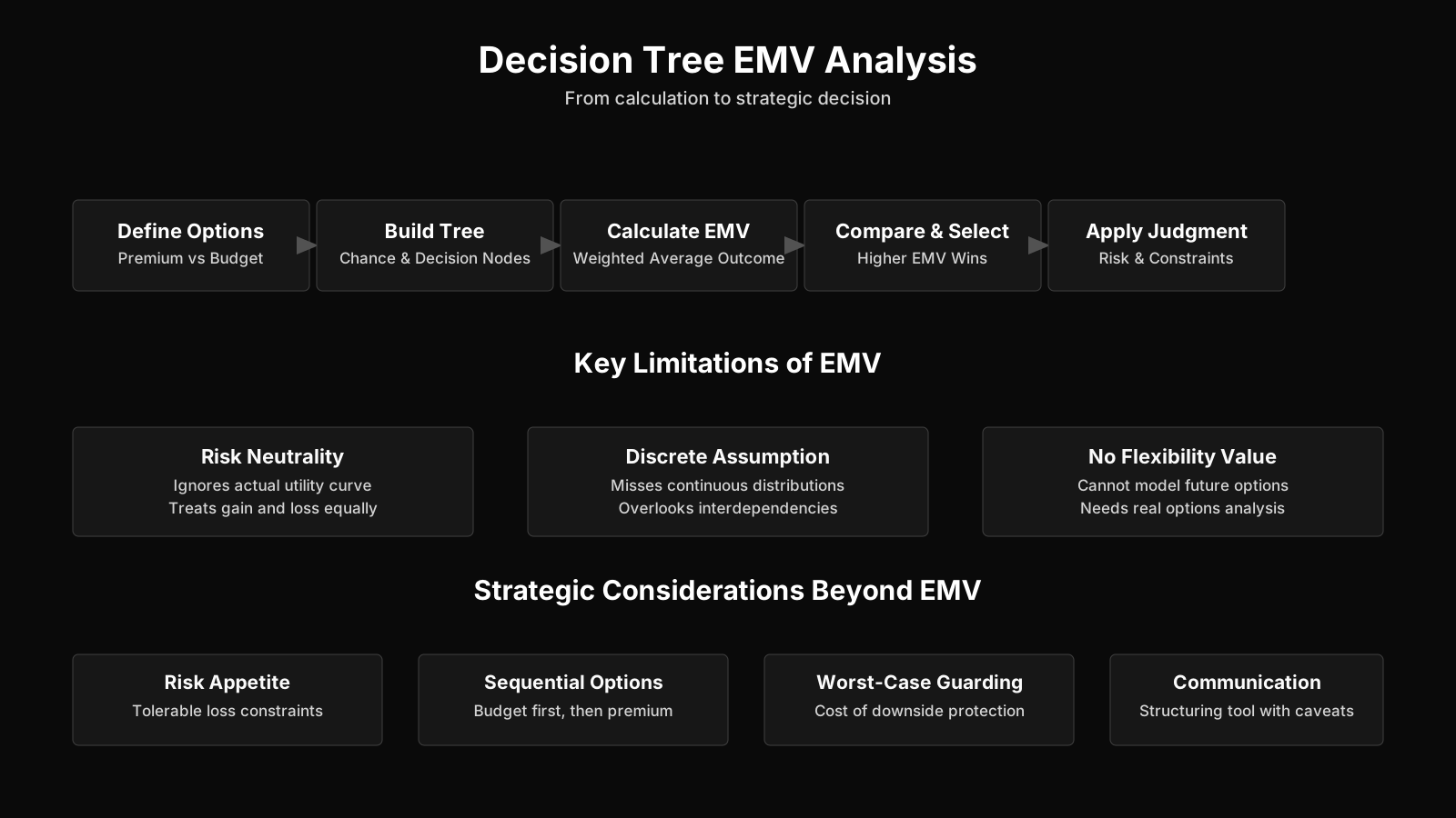
Key Steps to Calculate Expected Monetary Value with a Decision Tree
| Concept | Summary |
|---|---|
| Decision Tree Method | The decision tree maps sequential decisions and chance events into a single expected value per option, converting uncertain futures into comparable metrics for clear trade-off evaluation. |
| Expected Monetary Value (EMV) | EMV aggregates probability-weighted payoffs from all branches into a single figure, enabling decision makers to rank options by their average financial return and select the highest mean outcome. |
| Net Payoff Calculation | Every terminal branch reports the net cash that reaches the company's account, computed as gross revenue minus the upfront investment, reflecting the true financial gain or loss. |
| Illustrative Launch Scenario | The worked example pits a $40 million premium product launch against a $15 million budget version, showing how the tree surfaces the higher-expected-value path and informs the go/no-go decision. |
| Probability Nodes | The premium branch assigns equal 50 percent probabilities to high and low adoption outcomes; this deliberate simplification keeps the arithmetic transparent and the logic straightforward to verify. |
| Terminal Net Outcomes | Under high adoption, $110 million revenue yields a net payoff of $70 million after the $40 million investment. Low adoption results in $30 million revenue, producing a net loss of $10 million. |
| Expected Value for Premium | The tree yields a $30 million expected value for the premium launch, outweighing the $10 million loss in the low-adoption case and surpassing the budget alternative's lower but certain payoff. |
| Risk-Informed Decision Rule | A potential loss is not a disqualifier; it enters the weighted average as one data point, and because the combined expected value exceeds the budget launch's guaranteed floor, the decision maker rationally accepts the downside risk. |
Mapping the Product Launch Decision: A Step-by-Step Decision Tree
To ground the concept in something concrete, let’s build a decision tree for expected monetary value analysis from the bottom up. Imagine the company’s leadership in a conference room, a whiteboard covered with boxes and circles. The root node is a square labeled simply “Choose Launch Strategy.” From that square, two thick lines branch to the right. The upper line says “Premium Launch” with an investment of $40 million noted in small text. The lower line reads “Budget Launch” with a $15 million investment. Those investment figures are not part of the EMV calculation yet; they get folded into the net payoffs later. At the end of each decision branch sits a circle, the chance node, because neither launch guarantees a specific market response. The upper chance node, for the premium path, then splits into two terminal branches. The topmost branch corresponds to high market adoption, its probability scrawled next to it as 50 percent. That branch ends with a terminal value: a revenue of $110 million. But the decision tree must show net payoff, not gross revenue, so the whiteboard calculates $110 million minus the $40 million investment, yielding $70 million as the terminal outcome. The lower branch from that same premium chance node reflects low adoption, again with a 50 percent probability, and a revenue of $30 million. After subtracting the investment, the net payoff becomes a negative $10 million, equal to a loss. The budget side follows a similar pattern. Its chance node divides into high adoption, 50 percent probability, with $55 million revenue and a net of $40 million after the $15 million investment, and low adoption, 50 percent, with $25 million revenue netting $10 million.
The tree’s power is now evident: every scenario, every cash consequence, lies visible on a single sheet. No guesswork about forgotten combinations. The decision tree does not, however, tell you which branch to follow until you roll back the calculations from the endpoints toward the root. That rollback is where EMV enters.
Understanding Net Payoff Figures
One frequent source of confusion is the difference between revenue and net payoff. The decision tree terminal nodes must contain the net amount—the cash that actually lands in the company’s bank account after accounting for the upfront investment. For the premium launch, the high-adoption scenario grosses $110 million, but the net is $70 million because $40 million was spent to develop and market the product. That $40 million is not a future cash outflow; it is the sunk decision cost if the premium path is chosen. The tree assumes that once you commit to a branch, that cost is already incurred, so the terminal nodes represent incremental outcomes from that point. The budget launch’s high-adoption net of $40 million arises from $55 million revenue minus $15 million investment. On the low side, the premium launch brings $30 million revenue, which falls short of the $40 million investment, producing a $10 million loss, while the budget version still yields a positive $10 million net.
Probability Assignment and the 50 Percent Baseline
The example uses equal probabilities for high and low adoption, a deliberate simplification that keeps the arithmetic clean and the logic transparent. In real projects, probabilities would come from market research, historical data, or expert judgment. The key is that each chance node’s probabilities across all its branches must sum to 1.0, or 100 percent. Here, the 50-50 split satisfies that requirement, but the decision tree does not demand symmetry. The same EMV mechanics apply for any set of discrete outcomes, no matter how lopsided the probabilities.
Decision Tree Construction for Launch Payoffs
- Net payoff at terminal nodes
- Each terminal node represents the net financial return after subtracting the initial investment from expected revenue, as illustrated by a $70 million payoff for high adoption under a premium launch.
- Chance nodes for market response
- Both launch strategies lead to a chance node where high and low adoption each carry a 50% probability, reflecting the inherent uncertainty that no launch approach can guarantee a specific market outcome.
- Investment excluded from EMV calculation
- Upfront investment amounts, such as the $40 million premium launch cost, are not directly included in the EMV computation; they are already embedded within the net payoffs shown at each terminal node.
Crunching the Numbers: EMV Arithmetic for Premium and Budget Paths
The whole exercise culminates in computing expected monetary value with probability weights. EMV is elegantly straightforward: for each decision alternative, you multiply every possible net payoff by its probability and then sum the results. The sum represents the average financial outcome if the decision could be repeated many times under identical circumstances. Starting with the premium launch, you have two numbers: a 50 percent chance of $70 million and a 50 percent chance of negative $10 million. So the calculation is 0.50 times $70 million plus 0.50 times negative $10 million. This yields $35 million minus $5 million, equaling $30 million. That $30 million is the premium launch’s expected monetary value. For the budget launch, the arithmetic follows the same pattern: 0.50 times $40 million gives $20 million, and 0.50 times $10 million gives $5 million, summing to $25 million. The tree now carries these rolled-back EMV values at each decision node; the premium branch shows $30 million, the budget $25 million.
It is worth noting that the EMV of $30 million does not mean the company will actually get $30 million if it picks the premium launch. It will either gain $70 million or lose $10 million. The $30 million is a probability-weighted average, a mathematical abstraction that helps compare alternatives on an expected basis. In a world where the decision recurs many times, the average outcome would converge toward this number. For a one-shot project, the figure is still the risk-neutral benchmark. The budget launch’s $25 million EMV is lower, but notice both outcomes in that branch are positive; the worst case is a gain of $10 million. This absence of a loss scenario might appeal to a nervous CFO, though EMV as a pure number does not distinguish between risk profiles.
Double-Checking the Weighted Sums
A common error here is to inadvertently use gross revenues instead of net payoffs, which would bloat the EMV and skew the comparison. If you mistakenly multiplied 0.50 by $110 million and 0.50 by $30 million, you would get a premium EMV of $70 million, completely ignoring the investment. That would be a grave miscalculation. The tree forces you to place the net terminal values squarely, so the rollback respects the actual cash flow consequences.
Why the Premium Launch Wins Under Risk-Neutral Logic
With a $30 million EMV against a $25 million EMV, the EMV selection criterion in decision tree analysis points unequivocally toward the premium launch. The premium path offers an expected gain five million dollars higher than the budget alternative. That gap might seem small relative to the investment magnitudes, but in EMV terms it is decisive because every dollar of expected value counts. Risk neutrality—the assumption behind EMV—treats a dollar gained with the same utility as a dollar lost, evaluating decisions purely by their mathematical expectation. In this mindset, the possibility of a $10 million loss on the premium launch does not deter; it is simply a data point in the weighted average that still yields a higher mean than the budget launch’s riskless floor.
This is where many professionals pause. The premium launch literally opens the door to a net loss, whereas the budget launch guarantees some profit, albeit modest. A decision maker who is risk-averse might consciously override the EMV guidance and select the budget launch to sleep better at night. EMV as a concept does not incorporate such risk preferences; it is a cold arithmetic tool. That limitation does not invalidate the technique, but it demands that EMV be paired with a conversation about organizational risk appetite. For a well-capitalized company, the $10 million loss is a manageable downside that the expected upside more than compensates. For a firm operating on thin margins, that same loss could be catastrophic, rendering the EMV analysis moot.
The Influence of the Investment Size on the Decision
Notice that the premium launch’s larger investment of $40 million is both the source of its higher potential payoff and its lower floor. When the high-adoption revenue hits $110 million, the net is $70 million, dwarfing the budget’s $40 million net under the same scenario. But when adoption is low, the premium launch’s heavy upfront cost turns a middling revenue into a loss, while the budget launch’s lean cost structure still yields a surplus. EMV crystallizes these trade-offs. The decision tree also makes it easy to ask “what if” questions: what if the premium launch investment were $50 million instead? The net payoffs would shift, and the EMV might flip. This sensitivity is part of the tree’s ongoing value.
Core Insights on Risk-Neutral EMV Logic
- EMV criterion decisiveness
- The expected monetary value criterion unambiguously favors the premium launch, whose $30 million expected value surpasses the budget launch's $25 million by $5 million, a margin that eliminates any mathematical ambiguity.
- Risk neutrality core assumption
- Risk neutrality assumes that each dollar of gain and each dollar of loss carries identical utility, so decisions are evaluated solely by their mathematical expectation rather than by subjective attitudes toward losses or gains.
- Loss tolerance in weighted averages
- A potential $10 million loss does not deter a risk-neutral decision maker; it is merely one input in the probability-weighted average that, combined with more favorable outcomes, still delivers a higher mean return than the budget alternative.
- Risk appetite conversation needed
- A risk-averse decision maker may intentionally depart from EMV guidance to secure the budget launch's guaranteed modest profit, underscoring the need to complement quantitative EMV analysis with a structured discussion of organizational risk tolerance.
- Investment size dual effect
- The premium launch's $40 million investment simultaneously enables its higher potential payoff and creates its lower floor, making the scale of investment the central driver of the risk-return trade-off.
The Role of Probability in Shaping EMV and Decision Confidence
Because the EMV result hinges on two numbers multiplied, probability sensitivity in EMV decision trees deserves a hard look. The 50 percent probabilities are almost certainly approximations. What if the true likelihood of high adoption for the premium product is not a coin flip but something like 40 percent? Plugging a 0.40 probability into the premium EMV formula—0.40 times $70 million plus 0.60 times negative $10 million—yields $28 million minus $6 million, or $22 million. The budget EMV at that same 40 percent high-adoption rate becomes 0.40 times $40 million plus 0.60 times $10 million, giving $16 million plus $6 million, or $22 million, exact parity. At probabilities below 40 percent high adoption, the budget launch actually outperforms the premium launch in expected terms. This break-even probability threshold can be uncovered by solving the equation 80p minus 10 equals 30p plus 10, where p is the high-adoption probability. The solution is p equal to 0.40. So if the team judges high adoption to be more likely than 40 percent, the premium launch keeps its edge; otherwise, the budget version becomes the EMV favorite.
This kind of analysis transforms a static recommendation into a dynamic discussion. Project managers can present the decision tree not as a fixed answer but as a model that surfaces the assumptions that matter most. Stakeholders can then debate the probability estimate rather than argue about the final number. In cases where market research can tighten the probability estimate, the decision becomes sharper. When probabilities are truly unknowable, the break-even point at least frames the level of optimism required for the premium launch to be worthwhile.
Another nuance: the example uses only two possible outcomes per branch, which forces the team to collapse a continuous probability distribution into two bins. In reality, high adoption could be 30 percent, moderate 40 percent, low 30 percent, each with its own revenue and payoff. The decision tree handles multiple branches identically, though the mental load increases. The same EMV rollback logic applies, summing across all branches. The premium launch’s EMV might look different under a three-outcome model, but the fundamental mechanics do not change.
EMV Decision Trees Inside the PMBOK and Broader Frameworks
Within the PMBOK Guide, expected monetary value appears as a tool in quantitative risk analysis using expected monetary value, specifically under the Perform Quantitative Risk Analysis process in the Project Risk Management Knowledge Area. Decision tree analysis is listed as a technique alongside modeling and simulation methods like Monte Carlo. The PMBOK describes how you multiply the possibility of a risk event by its estimated impact in monetary terms, and how decision trees extend this to multiple future decisions and chance events. In that framework, the EMV of a risk response can be compared across alternatives, exactly as done with the premium and budget launch. The technique fits naturally into the planning phase, after risks have been identified and prior to selecting the risk response strategy that will be baked into the project budget and contingency reserves.
PRINCE2, the process-based project management methodology, also accommodates EMV thinking through its Risk Management Strategy, though it does not prescribe decision trees in the same explicit manner. The PRINCE2 emphasis on continued business justification means that the project board will evaluate options on a cost-benefit basis, often with expected values embedded in the business case. In agile environments, where the focus shifts to iterative value delivery and empirical validation, EMV calculations are less common but not obsolete. Large-scale agile frameworks sometimes use lean business cases that incorporate high-level expected value estimates to prioritize epics or feature sets. The decision tree’s visual nature complements the transparency agile teams value, even if the precise numbers are revisited frequently.
Monte Carlo simulation, another quantitative technique, can handle continuous distributions and complex interdependencies that a simple decision tree with discrete branches cannot. When a project has many interrelated variables, modeling thousands of scenarios with a computer often provides more realistic EMV estimates than a hand-built tree. That does not diminish the tree’s educational value; many risk workshops use decision trees first to build intuition before moving to simulation tools. The PMBOK also recognizes that EMV can be used in reserve analysis to set contingency reserves for known risks, where the sum of individual risk EMVs informs the budget buffer. So the ripple of EMV thinking extends beyond the immediate go/no-go decision into ongoing project financial governance.
Key Insights on EMV Decision Tree Use
- PMBOK quantitative risk analysis tool
- Within the PMBOK Guide, EMV is applied during the Perform Quantitative Risk Analysis process, where decision tree analysis serves as a modeling technique alongside Monte Carlo simulation to evaluate complex uncertainties.
- Probability multiplied by monetary impact
- The core EMV calculation multiplies a risk event's probability by its monetary impact, and decision trees build on this by structuring sequences of future decisions and chance nodes to value alternative paths.
- Planning phase and contingency reserves
- EMV integrates seamlessly into the planning phase following risk identification, and aggregating individual risk EMVs provides a quantitative foundation for reserve analysis when establishing contingency reserves for known risks.
- PRINCE2 business case alignment
- While PRINCE2 does not explicitly mandate decision trees, its principle of continued business justification encourages the use of expected monetary values in cost-benefit analyses to support the business case.
- Agile and simulation adaptability
- Agile frameworks rarely employ formal EMV analysis yet may incorporate rough estimates in lean business cases to help prioritize epics, while computer simulations of thousands of scenarios can yield far more realistic EMV figures than manually constructed decision trees.
Common Mistakes When Applying EMV Analysis
The technique is simple, which makes it dangerously easy to misuse. One of the common pitfalls in expected monetary value calculations is confusing gross revenue with net payoff, already touched on. Another is the failure to treat the investment as an incremental cost that must be applied to all branches of a given decision. Some teams will subtract the investment only from the low-adoption branch, reasoning that the high-adoption branch is profitable anyway. This distorts the EMV and leads to incorrect comparisons. The decision tree demands that the same investment be deducted uniformly across all outcomes tied to that decision point, because the cost is incurred regardless of the state of the world that follows.
Probability assignment errors also abound. Practitioners often pull probability figures from thin air, giving them an unwarranted precision. A 50 percent probability sounds scientific, but it might reflect nothing more than “we have no idea, so let’s call it even.” That level of uncertainty should be explicitly communicated and tested through sensitivity analysis, as earlier with the break-even point. Ignoring correlations between outcomes is another subtle trap. In the launch example, the high-adoption probability for the premium product might not be independent of the budget product’s performance; a booming market could lift both, while a recession could suppress both. The tree as drawn assumes independent chance nodes, which can overstate the diversity of outcomes. In reality, the two launch options might face the same underlying market factor, meaning the true variance is higher and the tree’s EMV may be overly optimistic in its risk aggregation.
Lastly, the pervasive error is treating EMV as the sole decision criterion. A $30 million EMV on a $40 million investment looks attractive, but it hides the fact that the company could lose $10 million 50 percent of the time. Risk-averse organizations or those with capital constraints cannot ignore that downside. Even the EMV’s assumption of risk neutrality is at odds with how real people in corporations behave. Many organizations supplement EMV with utility functions or minimum acceptable downside constraints, such as “no branch shall produce a loss greater than $5 million.” In such a filter, the premium launch would be rejected regardless of its superior EMV. Recognizing this human limitation is not a flaw of the technique but a necessity of its practical deployment.
Evolution of Decision Tree Value Analysis: BVOPM Perspectives
Modern methodologies like Business Value-Oriented Project Management, or BVOPM, push the boundaries of traditional EMV by integrating BVOPM quantitative risk and value into decision trees. In BVOPM, risk is not only expressed in monetary EMV but also tracked via standalone “Loss size” units, which quantify the magnitude of potential damage independently from probability. This dual lens allows a decision tree to display both the probability-weighted financial impact and the raw severity of a worst-case scenario. Additionally, BVOPM introduces Business Value Points, a composite metric that captures strategic, operational, and intangible benefits. For a product launch decision, the tree could augment the monetary branches with a Business Value Point trajectory, showing how each scenario contributes to market positioning, team learning, or future option value. The premium launch might score high on these points even in the low-adoption case because the R&D experience generates reusable knowledge, whereas the budget launch yields flat value points. Such augmentation does not replace EMV; it layers complementary information onto the same visual scaffold.
BVOPM also emphasizes process damage, a concept that tracks invisible erosion of team morale, technical debt, and stakeholder trust across different project paths. The decision tree in a BVOPM context might flag branches that carry high process damage, alerting decision makers that the EMV alone paints an incomplete picture. Meanwhile, the methodology’s dynamic filtering and frequent reassessment of Business Value Points allow the tree to be refreshed as the market evolves, moving the analysis from a one-time static snapshot to a living decision aid. This aligns with agile principles, though BVOPM remains agnostic about the delivery framework. For project managers accustomed to pure EMV, adding these dimensions may feel like extra work, but it addresses the very gaps that cause experienced managers to override the EMV recommendation. The result is a richer conversation around the whiteboard, one where the $30 million EMV is considered alongside a reminder that the premium branch’s process damage might be unacceptable, or that its Business Value Points could tip the scale even if the EMV gap narrows.
Key BVOPM Decision Tree Takeaways
- Dual risk quantification lens
- BVOPM evaluates risk through both probability-weighted monetary EMV and standalone Loss size units that quantify potential damage independently of probability, enabling decision trees to display financial impact and raw severity side by side.
- Business Value Points metric
- The composite Business Value Points metric captures strategic, operational, and intangible benefits such as market positioning, team learning, and future option value, and displays them as trajectories alongside monetary branches.
- Process damage and dynamic refresh
- Process damage tracks the invisible erosion of team morale, technical debt, and stakeholder trust, while dynamic filtering and frequent reassessment transform the decision tree into a living decision aid rather than a static snapshot.