Estimating the time and cost of project work sometimes feels like staring into a fog. You need numbers to build a schedule or a budget, but at an early stage you have little more than a rough scope. That is where parametric estimating enters the picture, offering a way to derive credible forecasts from historical patterns. In essence, parametric estimating uses a statistical relationship between historical data and other variables to calculate an estimate for activity parameters, such as cost, budget, and duration. To calculate a parametric estimate, you multiply the quantity of work to be performed by a known rate of labor hours or cost per unit. If history tells you that a designer can complete one drawing in eight hours, and you have 200 drawings to produce, the math points to 1,600 hours. This simplicity is deceptive because the real power, and the real challenge, lives in the quality of the data and the relevance of the relationship you choose.
The technique is not a guess dressed up in numbers. It rests on a measurable, repeatable connection between an independent variable, like square meters of concrete, lines of code, or meters of cable, and the effort or cost needed to produce it. Activity durations can be quantitatively determined by multiplying the quantity of work to be performed by labor hours per unit of work. The cable installation scenario is classic: 5,000 meters of cable at 0.15 labor hours per meter yields 750 hours of direct labor. If that rate is solid, the estimate is solid. If the rate was pulled from a project five years ago with a different crew and different site conditions, you are building your plan on sand. What makes parametric estimating attractive is also what makes it dangerous, a point we will return to again and again.
In the planning stages of a design project, the same logic applies. A project may require 350 design drawings, and organizational records show that each drawing consumed an average of 12 labor hours on past jobs of similar complexity. Multiply the two and you have 4,200 hours for drafting activity. The technique can produce higher levels of accuracy depending upon the sophistication and underlying data built into the model. If the model accounts for a fixed setup time, learning curves, or multiple drivers, it can become remarkably precise. But the model is only as good as the assumptions that feed it, and those assumptions need constant scrutiny.
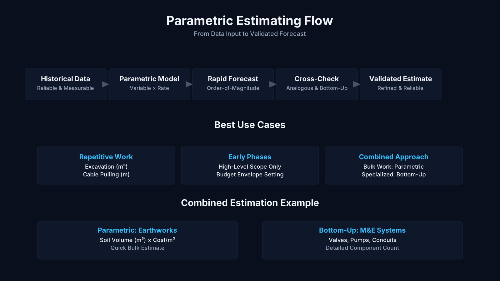
Parametric time estimates can be applied to a total project or to segments of a project, in conjunction with other estimating methods. You might use a bottom-up estimate for a complex integration task while leaning on a parametric model for repetitive installation work. This blending is common in infrastructure projects where earthworks can be estimated parametrically by cubic meters excavated, but building services must be detailed out component by component. The skill of the estimator lies in knowing when a parametric relationship holds and when it breaks down, something that is learned more through failure than through textbooks.
Quick Summary: How to Calculate a Parametric Estimate
| Key Concept | Summary |
|---|---|
| Parametric Estimating | Leverages statistical correlations between historical cost drivers and current project variables to produce scalable estimates for cost, schedule, and resource needs. |
| Independent Variables | Quantifiable factors such as concrete area, lines of source code, or cable length that serve as primary cost and effort multipliers for scaling estimates. |
| Historical Data | Benchmark metrics from past projects, like 12 labor hours per design drawing, provide the empirical foundation for parametric calculations. |
| Blended Estimation | Merges parametric scaling with detailed component breakdowns, applying distinct unit rates to disciplines such as structural frames, architectural finishes, and MEP systems. |
| Scale Effects | Productivity shifts non-linearly with project size; for instance, a painter’s coverage rate drops in expansive industrial halls due to increased travel time and logistical overhead. |
| Nonlinear Models | Sectors such as shipbuilding and software development rely on nonlinear parametric equations to model the exponential impact of project scale on cost and effort. |
| Overfitting Risks | Complex models can enhance accuracy but demand rigorous cross-validation and extensive data to avoid overfitting, which otherwise produces unreliable forecasts. |
| Resource Scheduling | Converting labor hours into calendar durations requires accounting for shift patterns, public holidays, and multitasking inefficiencies to avoid unrealistic timelines. |
Understanding the Parametric Estimate Formula
The core of any parametric estimate formula is the multiplication of a quantity by a unit rate. In its simplest form, E = Q × R, where E is the estimated effort or cost, Q is the quantity of work, and R is the historical rate per unit. This linear relationship is the most common entry point for project managers. But real-world work does not always scale linearly. There is often a fixed overhead component, like mobilizing a team or calibrating equipment, that exists regardless of quantity. A more nuanced model might be E = a + (b × Q), where a is a fixed setup effort, and b is the variable rate per unit. If historical data shows that setting up a test environment always takes 20 hours and each test case takes 0.5 hours, then 80 test cases would be estimated at 20 + (0.5 × 80) = 60 hours.
These incremental refinements matter enormously. The simpler linear model would have produced 40 hours, understating the true effort. The omission of fixed costs is one of the most frequent mistakes in parametric estimating. Teams that only track the unit rate and ignore the one-time activities end up with estimates that are consistently optimistic. The opposite trap is adding a fixed buffer arbitrarily without analyzing the data, which bloats estimates and erodes the credibility of the model. Statistical rigor is what separates a parametric estimate from a rule of thumb.
Nonlinear relationships also appear when economies of scale kick in or when complexity increases with volume. A painter who covers 30 square meters per hour on small rooms might only manage 20 square meters per hour on a vast, multi-level industrial hall because moving the scaffolding takes time. Parametric models can handle this by using a power function, such as E = a × Q^b, where b is less than 1 to represent efficiency gains. Deriving these models requires significant historical data and often regression analysis, but the increase in predictive accuracy can be substantial. Project managers in industries like shipbuilding or software development, where scale effects are pronounced, often rely on such nonlinear parametric models.
When multiple factors influence the outcome, multivariate parametric models come into play. A construction estimate might depend on the volume of concrete and the reinforcement density and the weather conditions. A cost model could be Total Cost = base + (rate1 × volume) + (rate2 × reinforcement weight) + (weather index factor). These models are built through multivariate regression on historical project data. The sophistication of the model increases the potential accuracy, but it also demands more data, more validation, and more vigilance against overfitting, where the model becomes so tailored to past data that it fails to predict new situations reliably.
Core Insights on Parametric Estimating
- Basic linear formula
- A straightforward parametric estimate that multiplies work quantity by a historical unit rate will underestimate the real effort unless fixed overhead items like site setup or team mobilization are accounted for separately.
- Fixed overhead inclusion
- One-time activities such as team mobilization and equipment calibration need to be explicitly added to the unit rate calculation, or the resulting estimate will be consistently optimistic because these unavoidable overheads are excluded.
- Model complexity trade-off
- More sophisticated formulas can sharpen accuracy, but they also demand larger datasets and stricter validation, while exposing the model to overfitting, a tendency that ultimately reduces the reliability of its forecasts on new projects.
Data Requirements for an Accurate Parametric Estimate
No model can rescue bad data, and this is where many parametric estimates go wrong. Historical data for parametric estimation must be clean, consistent, and truly comparable to the work being estimated. If a database shows that a particular task took 10 hours per unit, that number is only useful if you understand what was included in those 10 hours. Did it cover procurement, quality checks, rework, or just direct labor? A team that assumes the 10 hours includes everything may find that actuals double when indirect activities are added. This is a measurement definition problem, and it causes more estimating failures than any mathematical flaw.
Data normalization is the essential, unglamorous step that turns raw project logs into a reliable foundation. It means adjusting historical data for differences in team skill, tooling, location, and scope complexity. A rate of 2 hours per meter for cable pulling on a greenfield site with unobstructed trays cannot be applied directly to a brownfield retrofit where every meter involves navigating existing equipment. Normalization might involve applying a complexity factor or separating data into distinct project categories. Without this discipline, the parametric model becomes a garbage-in, garbage-out machine that undermines trust in the planning process.
The size of the historical dataset also influences confidence. A rate derived from three past projects will have a much wider confidence interval than one derived from thirty. Yet many organizations, especially smaller ones, have no structured archive of project performance data. They rely on anecdotal recollections or a single spreadsheet maintained by a long-tenured engineer. In such environments, parametric estimating is valid but requires extra caution. sensitivity analysis becomes crucial because you need to understand how much the estimate would change if the unit rate were 15% higher or lower. Running scenarios helps reveal whether the schedule or budget has any robustness at all.
Applying Parametric Estimates Across the Project Lifecycle
The application of parametric estimates changes as a project moves from initiation to execution. In the very early stages, when scope is still rough, a top-down parametric estimate can provide a ballpark figure that supports a business case or a portfolio decision. A program manager might estimate the cost of a new software module by multiplying the expected lines of code by a historical cost per line. That number, while imprecise, is often enough to compare investment options. As details firm up, the same parametric model can be recalibrated with more precise quantities and possibly split into work packages.
During detailed planning, parametric techniques are often used for specific types of work that lend themselves to unit measurement. Earthworks, concreting, cable laying, painting, and repetitive manufacturing steps are natural candidates. A project scheduler will take the quantity take-off from the engineering documents and convert it into durations using established productivity rates. This step is where parametric estimating interacts closely with resource loading. The duration estimate gives you labor hours, and the resource availability then translates that into calendar days, an additional layer that sometimes introduces errors if the team forgets to account for holidays, shifts, or multitasking.
Monitoring and controlling also benefit from parametric thinking. Earned value management compares planned value against earned value, which is often calculated using physical percent complete mapped to the same unit rates used in the estimate. If you budgeted 500 hours for 2,000 meters of cable and a progress measurement shows 1,200 meters installed with 400 hours spent, the parametric relationship immediately highlights a productivity issue. The cost performance index and schedule performance index gain meaning because the baseline was built on a defensible unit rate rather than a vague allocation.
Parametric Estimation for Activity Durations
When focusing on time, the formula flips from cost per unit to labor hours per unit, then to duration based on resource assignment. If a task requires 3,000 labor hours and you have five full-time workers, the duration would be 600 hours of elapsed work, or about 15 weeks at 40 hours per week, before considering other constraints. But here the parametric model is not just about multiplication; it must also respect calendaring realities. Non-working days, shift patterns, and resource ramp-up periods affect the actual elapsed time. In a design project, the number of drawings multiplied by the labor hours per drawing yields total effort, and the schedule then depends on how many designers are available and whether they can work in parallel without diminishing productivity due to communication overhead.
Teams often underestimate the effect of parallelization limits. The parametric labor estimate assumes a linear accumulation of effort, but adding more people to the same deliverables can reduce per-person efficiency due to coordination costs. This is not captured in a simple unit rate. A more sophisticated parametric model for duration might include a factor for team size efficiency, derived from past project data showing how productivity per person drops as the team grows. Such a model moves beyond the basic E = Q × R and starts to reflect the realities of knowledge work and heavy engineering alike.
Parametric Estimation for Project Costs
Cost estimation through parametric models follows the same logic, with the unit rate expressed in monetary terms per unit of output. A commercial interior fit-out might have historical data showing a cost of $1,200 per square meter for a standard specification. To estimate a 1,000 square meter office, you multiply to get $1.2 million. But what about location adjustments, material price escalation, and design complexity? Just as with durations, cost models need normalizing factors. A parametric cost estimate that ignores the difference between a city center site with delivery restrictions and a suburban site with easy access will be dangerously inaccurate.
Cost models can also include component breakdowns within the same parametric framework. Instead of a single blended rate per square meter, the estimate might use rates for structural elements, finishes, and MEP (mechanical, electrical, plumbing) separately, each derived from historical jobs. This layered approach improves traceability and makes it easier to adjust the estimate when a stakeholder asks, “What if we downgrade the floor finishes?” Because the cost drivers are separated, the impact of a change can be isolated, which is far harder to do with a black-box blended rate.
Key Insights on Parametric Estimating
- Early Top-Down Estimates
- During early scoping, parametric formulas generate rapid, high-level estimates that inform business cases and portfolio selection long before detailed scope is defined.
- Rebasing as Scope Firms
- As scope firms up, the same parametric model can be recalibrated with refined quantities and disaggregated into work packages for earthworks, concreting, cable laying, and repetitive manufacturing tasks.
- Converting Quantities to Durations
- Project schedulers convert engineering quantity take-offs into labor hours using established productivity norms, which then underpin the calculation of activity duration estimates.
- Resource Availability Adds Complexity
- Converting labor hours into calendar days demands careful factoring of assigned crew sizes, holidays, shift patterns, and multitasking, a step where scheduling errors most commonly arise.
- Detecting Productivity Issues
- Comparing actual progress against the parametric budget, for instance 400 hours spent to lay 1,200 meters of a 2,000-meter cable run, quickly reveals productivity shortfalls and prompts corrective action.
Accuracy, Limitations, and Common Misconceptions
The promise of accuracy of parametric estimates can be a trap if the limitations are not fully acknowledged. The technique can produce valid ranges, but it is not a crystal ball. One pervasive misconception is that parametric estimating eliminates uncertainty. It does not. The unit rate itself is a random variable with a distribution, not a fixed constant. A proper parametric estimate should be expressed as a range, perhaps with a most likely value and optimistic and pessimistic bounds derived from the historical standard deviation of the unit rate. Project managers who present a single deterministic number from a parametric calculation are doing their stakeholders a disservice.
Another common error is assuming that the relationship is causal. A high correlation between two variables in past data does not mean that one drives the other, yet parametric models are often built on such superficial associations. For example, a dataset might show that projects with more pages of documentation took longer, so a model might add a factor for page count. But the real driver might be stakeholder review cycles, which both increase page count and extend duration. If the project changes its review process, the page-count relationship collapses. A responsible parametric model is grounded in domain understanding, not just statistical coincidence.
Parametric estimating also struggles with novelty. When a project includes a component that has never been done before, there is no historical unit rate. Attempting to force a parametric relationship by analogy with a loosely similar activity is risky. A new chemical process unit may be measured in throughput capacity, but using the cost-per-ton rate from a decades-old plant of a different technology will mislead. In these cases, parametric estimates must be complemented by expert judgment or bottom-up analysis, and the assumptions need to be flagged prominently so that decision makers understand the fragility of the numbers they are using.
Parametric Estimating Across Different Methodologies
Formal project management frameworks give parametric estimating specific homes. In the PMBOK Guide, parametric estimating in project management appears as a tool and technique within the Estimate Activity Durations and Estimate Costs processes, both part of the Planning Process Group. The guide highlights its reliance on a statistical relationship and notes that it can be applied at different levels of detail. This endorsement means that many organizations standardize their estimating practices around parametrics, and the associated project management software often includes fields for unit rates and quantities, making the technique easy to apply mechanically, though not necessarily easy to apply well.
PRINCE2 does not explicitly name parametric estimating but embeds estimation within its Plans theme, where multiple techniques are accepted. The emphasis in PRINCE2 on product-based planning means that the quality of the product description and the breakdown of work products naturally create a structure for applying parametric rates. A project manager building a product flow diagram can assign effort or cost per product type using historical data, which is a parametric approach in all but name. The difference is one of terminology rather than concept, and a PRINCE2 practitioner will find the mathematical underpinnings of parametric estimation entirely compatible with the framework’s principles.
Agile environments at first glance seem distant from parametric models because scope emerges and work is sized in story points. Yet parametric thinking sneaks in through velocity. A team’s historical velocity, say 30 story points per sprint, is a unit rate, and the product backlog size is the quantity. Dividing backlog points by velocity gives a rough number of sprints, which translates to a duration estimate. This is not a pure parametric estimate because story points are relative and not tied to a fixed unit of physical output, but the structural logic is the same. Some Agile teams go further by tracking cycle times and using historical average cycle times per story point as a parametric duration predictor, blurring the line even more.
Core Takeaways on Estimating Frameworks
- PMBOK explicit endorsement
- The PMBOK Guide explicitly identifies parametric estimating as a core technique for Estimate Activity Durations and Estimate Costs within the Planning Process Group, underscoring that its reliability hinges on statistically valid correlations between historical data and project parameters.
- Standardized software integration
- Formal endorsement by PMBOK has led many organizations to standardize on parametric methods, with project management tools now routinely embedding unit rate and quantity fields that streamline data entry and reduce application overhead.
- PRINCE2 implicit adoption
- While PRINCE2 never names parametric estimating, its Plans theme weaves estimation directly into product-based planning, creating a natural structure for applying unit rates derived from historical data sets.
- Product flow diagram rates
- When building a product flow diagram, a PRINCE2 manager can assign effort or cost per product type using historical benchmarks, which amounts to a parametric approach in practice even without the formal label.
- Agile structural similarity
- Agile story points offer relative sizing that is not tied to fixed physical output, so they are not a pure parametric estimate, yet the underlying principle of quantifying work through a calibrated, scalable measure mirrors the same logical foundation.
Refining Your Parametric Estimate Models Over Time
A parametric model is not a set-and-forget artifact. Refining parametric estimate models is a continuous activity that pays off most when organizations treat every completed project as a data source to update their estimating database. Recalibration involves comparing the parametric estimate made at the planning stage with the actual outcome, computing the variance, and investigating whether the unit rate, the quantity, or the model structure was at fault. If a concrete pour productivity rate turns out to be 15% slower than the historical average on three consecutive projects, the central rate should be adjusted, not explained away.
Feedback loops also help capture missing variables. A project that consistently overruns its parametric estimate may reveal a hidden complexity driver that never appeared in the original model. Perhaps the rate per installation should be segmented by floor height because high-level work takes longer. Such insights flow from comparing planned versus actual at the work package level and drilling into the root causes. This practice converts parametric estimating from a static technique into a learning system, an approach that aligns well with the iterative improvement mindset of many modern management philosophies.
The statistical tools used for model refinement are not exotic. Simple linear regression on updated datasets, calculation of R-squared values to assess fit, and residual analysis to check for patterns all fall within the reach of most project management offices. The barrier is not mathematics; it is organizational discipline. Parametric models degrade when nobody maintains them, when rates become folklore rather than verified numbers, and when the culture rewards hitting the estimate more than improving the estimate. A project team that is never asked to explain an estimating error will never feed back the data needed to sharpen the model.
Connecting Parametric Estimating to Value-Driven Approaches
Modern methodologies that emphasize business value offer a different lens on estimation. In Business Value-Oriented Project Management (BVOPM), planning practices incorporate parametric estimating in value-driven planning but treat it with caution. BVOPM promotes relational effort points over deterministic unit rates and explicitly warns that detailed work breakdown structures can accumulate inaccuracies that weaken parametric models. The philosophy is that scope should be allowed to evolve based on feedback, so locking an estimate to a fixed quantity early on is counterproductive. Instead, parametric relationships serve as initial sizing tools, and the plan adapts as the team discovers more about the work and its value.
BVOPM’s treatment of scope change as user feedback rather than failure reshapes how parametric estimates are used. When a stakeholder requests a feature that changes the quantity in the formula, the estimate is not discarded but is dynamically updated, and the conversation shifts to value prioritization rather than schedule defense. This approach reduces the adversarial dynamic that often surrounds parametric estimates in traditional governance, where any deviation from the original quantity can be seen as a planning failure. It does not, however, eliminate the need for solid data; the relational effort points still need calibration against past delivery data, keeping the parametric spirit very much alive.
Value-Driven Estimation Key Insights
- Caution in value-driven planning
- BVOPM applies parametric estimating during value-driven planning while remaining careful about the reliability of deterministic unit rates.
- Relational effort points preferred
- The method favors relational effort points over fixed unit rates to circumvent the compounding errors that arise from finely granulated work breakdown structures.
- Scope evolves from feedback
- Because fixing an estimate to a rigid quantity too early undermines adaptability, parametric relationships serve solely as preliminary sizing tools.
- Estimates update dynamically
- As scope adjustments modify the underlying quantities, estimates are recalibrated instead of abandoned, redirecting discussions toward value-based trade-offs.
- Data calibration remains vital
- Relational effort points must still be calibrated with historical delivery data, maintaining a parametric discipline within adaptive planning contexts.
Common Pitfalls When Calculating Parametric Estimates
Avoiding the pitfalls in parametric estimating requires more than awareness, it demands explicit process steps that catch errors before they become baselines. One of the most seductive mistakes is cherry-picking the unit rate. An estimator may look at a spread of historical productivity figures and select the best-case rate because the project sponsor wants an aggressive target. This is basically anchoring on optimism. Over time, a portfolio of such estimates creates a systemic bias where plans are consistently unachievable, leading to firefighting, overtime, and stakeholder mistrust. Forcing the use of a weighted average or a P50 value, and documenting the rationale, can mitigate this.
Scope creep also fatally wounds parametric estimates when the quantity grows but the rate is not reapplied. A common pattern is that a parametric estimate is built at a conceptual level with 400 units. Through design development, the quantity becomes 550, but the schedule and budget are not recalculated using the original parametric formula. Instead, a flat percentage is added, which may not reflect the true marginal cost or effort. The remedy is to keep the parametric model alive as a living document that is refreshed whenever the quantity baseline changes, something that requires strong version control and a culture that respects the model’s integrity over political convenience.
There is also the pitfall of confusing precision with accuracy. A parametric model can generate a number like 1,847.5 hours, which looks precise, but the underlying uncertainty might be plus or minus 40%. Decision makers latch onto the precise figure, ignoring the wide confidence interval. Communicating estimates as ranges with confidence levels is not just good practice; it is an ethical obligation for the estimator. When a project manager says, “Based on historical data, the duration will be between 24 and 38 weeks with 90% confidence,” the conversation shifts from false certainty to risk management, which is exactly where it should be.
Parametric Estimating and the Broader Estimating Toolkit
No project is estimated with a single technique. Calculating parametric estimates alongside analogous and bottom-up methods creates a cross-check that improves overall credibility. Analogous estimating, which uses the cost or duration of a similar past project as a whole, provides a fast top-down sanity check. If the parametric model for a new highway segment comes back at $22 million, but an analogous segment built last year cost $30 million, that discrepancy forces an investigation. The parametric model might be missing a major cost element, or the analogous comparison might be distorted by unique circumstances. The triangulation process strengthens the final number.
Bottom-up estimating, where each work package is estimated in detail and rolled up, often serves as the final baseline. But parametric estimates can feed those bottom-up cells. A work package for “installation of 200 lighting fixtures” might be bottom-up in structure but parametric in its underlying rate calculation because the estimator uses a standard labor hour per fixture times the quantity. The distinction blurs. So rather than viewing techniques as competitors, seasoned project managers treat them as layers of an onion, with parametric providing the rapid outer layers and bottom-up adding granularity as the project definition sharpens.
The interaction with three-point estimating is particularly powerful. For each parametric unit rate, an optimistic, most likely, and pessimistic value can be gathered from historical distributions. Then the estimate is run through Monte Carlo simulation to produce a probability curve. This transforms the parametric model from a single-point estimate into a stochastic forecast that speaks directly to the project’s risk appetite. It is a natural marriage of parametric logic and quantitative risk analysis, and one that many organizations underutilize simply because they have not invested in digitizing their historical rate data with dispersion measures, not just averages.
Core Insights on Estimate Layering
- Cross-checking techniques boosts credibility
- Rarely is a project estimated using a single method; seasoned managers combine parametric, analogous, and bottom-up approaches to triangulate reliable figures, creating a cross-check that significantly enhances overall credibility.
- Discrepancies trigger valuable investigations
- A sharp divergence, such as a parametric estimate of $22 million versus an analogous estimate of $30 million for a comparable highway segment, forces teams to investigate whether a critical cost element was overlooked or if unique project circumstances distorted the comparison.
- Layered methods sharpen risk forecasting
- Treating estimation techniques as complementary layers transforms parametric models from static single-point forecasts into stochastic analyses aligned with risk appetite, though many organizations underutilize this potential because they lack digitized historical rate data that includes dispersion measures.
Evolving the Practice of Parametric Estimation
The discipline is not static. As organizations adopt more data-driven project management, the future of parametric estimate calculation points toward greater automation and machine learning integration. Predictive analytics platforms can now ingest project data from dozens of completed efforts, automatically identify the most predictive variables, and suggest parametric models with confidence bands. This reduces the reliance on the lone estimator’s spreadsheet and spreads the knowledge across the organization. However, the human chore of validating the logic, questioning spurious correlations, and ensuring the data is normalized remains irreplaceable.
Another evolution is the shift from project-level parametrics to portfolio-level parametrics. A PMO can build models that estimate the total capacity needed for a pipeline of projects based on historical ratios of effort per dollar of capital, or duration per thousand square meters. This enables strategic workforce planning and capital allocation decisions with far more rigor than simple trend extrapolation. A portfolio manager who can say, “Based on our parametric model, the proposed program will require 400,000 engineering hours over three years,” provides a fact-based foundation for executive decisions.
The human element, though, will always be the limiting factor. A parametric model that is politically rejected because its findings are inconvenient is worthless. Building trust in the model means involving the project delivery teams in its creation and calibration. When the engineers who perform the work agree that the unit rates are realistic given their constraints, they are far more likely to commit to the resulting schedule. Conversely, a model handed down from a central planning group without consultation will be ignored or blamed when things go wrong. The social engineering of estimation acceptance is just as important as the statistical engineering.
Ultimately, parametric estimating endures because it connects the ambition of a plan to the evidence of what has been accomplished before. It replaces subjective optimism with data, or at least forces the optimism to be quantified as a variance from the historical norm. For a project manager standing at the start of a complex endeavor, a well-constructed parametric model is not a guarantee of success, but it is a compass that points in a direction worth exploring. And when it is wrong, as it sometimes will be, the error itself becomes one more data point that makes the next estimate that much sharper.