Risk analysis depends on probability distributions to translate uncertain estimates into meaningful ranges of possible outcomes. The common probability distributions for risk analysis include continuous distributions such as beta, triangular, uniform, normal, and lognormal, along with discrete distributions for events and scenarios. These distributions allow project teams to model uncertainty in schedule durations, cost components, and decision tree branches without pretending that a single point estimate captures reality. In a quantitative risk model, a distribution is not a side detail; it is the mathematical representation of what the project knows and does not know about a particular variable.
Continuous probability distributions appear frequently in Monte Carlo simulation and other modeling techniques because schedule durations and cost components rarely behave as fixed values. Discrete distributions handle different kinds of uncertainty, such as whether a test passes or which branch of a decision tree materializes. Together they give project risk practitioners a structured way to move from single point estimates to a range of possible outcomes with associated likelihoods.
Key Probability Distributions for Risk Analysis: A Summary
| Distribution Types | Analytical Summary |
|---|---|
| Continuous Distributions | Continuous distributions model variables that can assume any value within a specified range, including task durations, resource effort, and component costs, making them suitable when intermediate values are plausible. |
| Discrete Distributions | Discrete distributions represent variables with a finite or countable set of outcomes, such as pass/fail states, defect counts, and decision tree branches, where fractional values would carry no practical meaning. |
| Appropriate Distribution Selection | Selecting the correct distribution type is foundational because applying a continuous curve to a limited set of discrete outcomes produces fractional results that distort the analysis. |
| Chart Interpretation | Reading a distribution chart requires assessing how probability is spread across possible values rather than interpreting the curve as a trend over time. |
| Simulation Sampling | Simulation software repeatedly draws random samples from the fitted distribution to generate probabilistic ranges for project completion dates and total cost outcomes. |
| Risk Analysis | A risk analyst who understands the selected distribution can calibrate its parameters to reflect expert judgment more accurately than a default triangular distribution. |
| Beta Distribution | The beta distribution is particularly useful when experts can supply a credible minimum, a maximum, and a most likely value within that range. |
Common Probability Distributions for Risk Analysis: Continuous and Discrete Types
In risk analysis, continuous probability distributions for time and cost uncertainty are used extensively in modeling and simulation. Continuous distributions apply when a variable can take any value within a range, such as an activity duration of 23.7 days or a component cost of 14,320 currency units. They form the mathematical backbone of Monte Carlo simulation because they allow the model to generate thousands of plausible values between specified bounds. Discrete distributions, by contrast, represent uncertain events that have a limited number of outcomes, such as the outcome of a test or a possible scenario in a decision tree.
Discrete distributions assign probability masses to specific outcomes rather than spreading probability across a smooth curve. A binary pass/fail condition, a chance branch in a decision tree, or a limited set of regulatory outcomes all fit naturally into a discrete distribution. Choosing the correct type is a foundational step because a continuous curve applied to an event with only a few outcomes will produce meaningless fractional results. A discrete distribution applied to a variable that can take any value within a range will similarly miss the nuance of partial values.
The horizontal X axis of a probability distribution chart represents possible values of time or cost. The vertical Y axis represents relative likelihood. When a team reads a distribution chart, they are not looking at a schedule or a budget line; they are seeing how probability is spread across the range of potential values. That visual shift is often harder than it sounds because many people instinctively read a rising curve as a trend over time when it actually shows how likely each value is.
Continuous Common Probability Distributions for Risk Analysis
Within schedule and cost modeling, continuous distributions represent the uncertainty in values such as durations of schedule activities and costs of project components. A project manager may estimate that a specific engineering task will take between 20 and 40 days, with some values more likely than others. The continuous distribution captures that entire range instead of forcing the model to use a single deterministic number. In a simulation, the software samples from this distribution repeatedly, producing a range of possible project completion dates and total costs.
Many quantitative risk models combine several continuous distributions. One activity may use a triangular distribution while another uses a beta distribution, depending on the shape of uncertainty. This mixing is normal as long as the distribution choice matches the underlying estimate. The risk register and the project schedule provide the data inputs, but the distributions define how that data behaves under uncertainty.
Discrete Probability Distributions in Risk Analysis
Discrete distributions become essential when modeling events that either happen or do not happen. A regulatory approval may have a 70 percent chance of success and a 30 percent chance of delay. A decision tree branch may lead to one of three possible scenarios, each with an assigned probability. In these cases, a continuous curve would be misleading because the variable cannot take intermediate values like 0.5 of an approval.
Practitioners sometimes overlook discrete risk events because they focus on cost and schedule ranges. That is a mistake. Event risks can trigger major changes to the project plan, and their probabilities often drive the shape of contingency reserves. Combining discrete event distributions with continuous impact distributions creates a more complete picture of overall project risk exposure.
Essential Summary: Distribution Types
- Continuous distributions in simulations
- Continuous distributions represent variables that can assume any value within a given range, such as durations or costs, and they serve as the foundation of Monte Carlo simulation by producing thousands of credible scenarios.
- Discrete distributions for limited outcomes
- Discrete distributions allocate probability mass to a finite set of distinct outcomes, which makes them well suited for modeling pass/fail results, decision tree branches, and limited regulatory scenarios.
- Matching distribution to problem
- Selecting the appropriate distribution type is essential because forcing a continuous curve onto a small number of discrete outcomes yields meaningless fractional values that do not correspond to any real-world state.
- Reading distribution charts
- A distribution chart illustrates how probability is dispersed across possible values rather than how a variable changes over time, and rising curves in these charts often mislead viewers into reading them as time trends.
- Sampling for project outcomes
- Simulation software draws repeated samples from the selected distribution to generate a realistic range of potential completion dates and total project costs, reflecting the underlying uncertainty in each input.
Beta Distribution for Risk Modeling
The beta distribution is one of the most frequently used continuous distributions in project risk analysis. Its popularity comes from flexibility. The beta distribution shape parameters determine whether the curve is symmetric, skewed left, skewed right, or nearly flat. Two shape parameters, traditionally labeled alpha and beta, control the curve's form. That flexibility allows a risk analyst to model an estimate where the most likely value sits closer to the optimistic end or closer to the pessimistic end.
In practice, the beta distribution often appears in PERT-style estimates. PERT traditionally uses a weighted average of optimistic, most likely, and pessimistic values. The beta distribution builds on that three-point logic but allows a richer representation of uncertainty. For example, a task duration with an optimistic estimate of 10 days, a most likely estimate of 15 days, and a pessimistic estimate of 35 days will have a right-skewed shape because the pessimistic tail is longer. A symmetric beta curve would be inappropriate for that kind of estimate.
One common misconception is that the beta distribution always looks like a smooth bell. It does not. Depending on the shape parameters, the beta distribution can take on U shapes, J shapes, or rectangular forms within a bounded interval. That is why it is so useful for bounded variables like duration and cost. The distribution remains within a defined minimum and maximum, which matches the way many project estimates are expressed.
Think of the two shape parameters as dials that bend the curve toward either end of the estimation range. If the dials are equal and greater than one, the curve humps in the middle. If one dial is larger, the curve leans toward that side. A risk analyst who understands this can fine-tune the distribution to reflect expert judgment more accurately than a simple triangular curve might allow.
When to Use the Beta Distribution in Risk Analysis
The beta distribution works well when experts can provide a minimum, a maximum, and a sense of where the most likely value falls within that range. In schedule risk analysis, activities with moderate asymmetry benefit from beta modeling. Cost items that are bounded by contractual limits or physical constraints also fit naturally. The key advantage is that the beta distribution does not assume symmetry, so it can represent realistic skew in project data.
However, selecting appropriate shape parameters can be tricky. PERT formulas provide one approach, but many simulation tools allow the analyst to adjust the parameters manually. Without good historical data, the choice can feel subjective. Even so, a well-informed beta distribution usually outperforms a single point estimate or a crude normal assumption for bounded project variables.
Triangular Distribution for Schedule and Cost Risk
The triangular distribution is another frequently used continuous distribution in risk analysis, largely because it is simple and intuitive. Triangular distribution for schedule and cost risk relies on three parameters: a minimum value, a most likely value, and a maximum value. The resulting shape is a triangle with its peak at the most likely value. This simplicity makes it attractive when detailed historical data is unavailable and the project team must rely on expert judgment.
In practice, a project controller might say that procuring a specialized component will cost between 50,000 and 90,000 currency units, with a most likely cost of 65,000. The triangular distribution turns those three numbers into a probability curve. The probability rises linearly from the minimum to the most likely value, then falls linearly to the maximum. No other parameters are required, which means the model can be built quickly and explained easily to stakeholders.
That ease of explanation is not trivial. Project risk workshops often include people who are not statisticians. When a facilitator draws a triangle and labels the three points, participants can immediately see how their estimate translates into a risk profile. A beta distribution may be more flexible, but explaining its shape parameters in a workshop can slow things down. The triangular distribution trades some mathematical refinement for clarity and speed.
The main limitation of the triangular distribution is that its sharp peak can overemphasize the most likely value. Real-world uncertainty is often smoother. It also places zero probability exactly at the minimum and maximum, which may not reflect reality if the bounds are soft. Despite these limitations, the triangular distribution remains widely used because it provides a reasonable first approximation in many project risk models.
Some practitioners note that the triangular distribution can create artificial tails if the bounds are chosen poorly. If an expert sets the maximum far higher than realism to be safe, the triangle flattens and spreads probability over an improbable range. That can inflate the simulated risk exposure. The solution is not to abandon the triangular distribution but to challenge the three input values during the risk workshop.
Three Point Estimates and Distribution Shape
Three point estimates feed naturally into triangular distributions. The optimistic, most likely, and pessimistic values are already common language in project planning. The triangular distribution simply formalizes the uncertainty between those points. This connection to familiar estimating techniques is one reason the distribution appears so often in quantitative risk analysis templates and software defaults.
When using the triangular distribution, the risk analyst should avoid treating the three points as deterministic truth. They are judgment calls. The distribution only translates those calls into a consistent probabilistic form. If the underlying three point estimates are biased, the resulting distribution will inherit that bias. Good risk facilitation therefore focuses as much on calibrating expert judgment as on selecting the distribution shape.
Essential Summary of Triangular Risk Modeling
- Three parameter inputs required
- The triangular distribution requires only a minimum, most likely, and maximum value to define a complete risk profile for schedule or cost items.
- Ideal for expert judgment situations
- When historical data are scarce, this distribution converts straightforward expert judgments into a defensible probability curve that supports decision making without extensive records.
- Fast, transparent stakeholder communication
- Because the model requires no additional parameters, facilitators can sketch the triangle directly and immediately show participants how their estimates translate into risk exposure.
- Caution against inflated maximum values
- If an expert sets an unrealistically high maximum to appear conservative, the triangle flattens and spreads probability across an implausible range, which can materially distort the risk profile and downstream decisions.
Uniform Distribution in Early Concept Risk Analysis
A uniform distribution is used only if there is no obvious value more likely than any other between specified high and low bounds. Uniform distribution for bounded but uncertain estimates is particularly relevant in the early concept stage of design, when detailed information is scarce. If a team knows that a new facility might cost between 2 million and 3 million currency units but has no basis to favor any part of that range, a uniform distribution assigns equal probability to every value in between.
This distribution is flat, with a constant likelihood across the entire interval. It does not imply that the midpoint is more likely, nor does it create a peak. That property distinguishes it sharply from triangular, beta, and normal distributions. The uniform distribution says something quite specific: the team is equally uncertain across the full range. Using it when some values genuinely are more likely than others would misrepresent the available knowledge.
Many project teams resist the uniform distribution because it feels too crude. But in early stages, pretending to know more than you do is a real risk. A uniform distribution can actually be the most honest representation of deep uncertainty. It prevents the model from pretending that a most likely value exists when the team has not yet gathered enough information to identify one.
What this means in practice is simple. If an engineer says a new process could take anywhere from 12 to 18 weeks and truly cannot narrow that range, the uniform distribution reflects that ignorance without inventing a false peak. The simulated schedule will show a broad spread of possible completion dates, which is exactly what the current state of knowledge supports. As more design information becomes available, the team can replace the uniform distribution with a more shaped distribution.
One pitfall is using the uniform distribution as a lazy default simply because the team did not bother to think through the shape of uncertainty. That is different from a deliberate decision based on genuine lack of information. The distinction matters because the uniform distribution spreads probability evenly, which can either honestly reflect ignorance or artificially hide a known tendency toward certain values.
When No Value Is More Likely Than Another
The phrase "no obvious value more likely than any other" is the key test for the uniform distribution. If the project team can point to a reason that one part of the range is more plausible, they should not use a uniform distribution. Early concept design work often meets this test because many technical and commercial factors remain unresolved. At that stage, broad equal uncertainty is a reasonable starting assumption.
Uniform distributions also appear in sensitivity analysis and scenario modeling when analysts want to explore the full range without imposing assumptions. That exploratory use is valid, but the results should be interpreted as bounds, not as predictions. The flat curve does not forecast the future; it simply maps the space of current possibilities.
Normal Distribution for Symmetric Risk Variables
The normal distribution is widely recognized and sometimes overused in risk analysis. Normal distribution for symmetric variability is appropriate when deviations from a central value are equally likely in both directions and the variable can theoretically extend indefinitely in either direction. The bell-shaped curve peaks at the mean, with probability tapering off symmetrically on both sides.
In project risk analysis, normal distributions can model measurement errors, certain performance metrics, or aggregated effects where many small influences combine. If a manufacturing process has a target cycle time with small random variations above and below that target, a normal distribution may fit reasonably well. The same logic can apply to some cost estimating errors when historical data shows a balanced spread around the estimate.
However, the normal distribution has important limitations for project variables. Schedule durations and costs cannot be negative, but the normal distribution has no natural lower bound. It allows a small probability of negative values unless truncated. More importantly, many cost and duration uncertainties are skewed rather than symmetric. A task is more likely to overrun than to finish far earlier than expected, and that asymmetry violates the normal assumption.
Despite these drawbacks, the normal distribution remains common in risk workshops because people understand the bell curve. That familiarity can be dangerous if it leads to mechanical use without checking the shape of the data. A risk analyst should ask whether the variable truly is symmetric and unbounded before applying a normal distribution. In many bounded project contexts, beta or triangular distributions are more defensible.
Using Normal Distribution for Aggregated Project Risk
One valid use of the normal distribution arises when aggregating many independent risks. The central limit theorem suggests that the sum or average of many small random effects tends toward a normal shape, even if the individual effects are not normal. In project cost risk, the combined effect of many minor uncertainties may approximate a normal distribution around the expected total cost. This can support high-level portfolio analysis, though the tails may still be underestimated.
Practitioners should be cautious about extrapolating normal results to extreme tails. Project risk management often focuses on rare but severe outcomes, exactly where the normal curve assigns very low probability. If historical data show fat tails, a lognormal or other skewed distribution may better capture the risk of large overruns. Relying on the normal distribution in those situations can produce dangerously optimistic contingency reserves.
Core Takeaways on Normal Risk Modeling
- Symmetric deviation application
- The normal distribution is appropriate when positive and negative deviations from a central value are equally probable and the variable can, in principle, extend indefinitely in either direction.
- Limitations for project metrics
- Schedule durations and costs are bounded at zero, and project tasks tend to overrun far more often than they finish early, so the symmetric normal curve misrepresents these practical realities.
- Persistent workshop popularity
- Although the normal distribution assigns very low probability to the rare, high-impact outcomes that project risk management most needs to anticipate, it remains widely used because stakeholders find the bell curve intuitive and accessible.
Lognormal Distribution for Skewed Project Risks
The lognormal distribution is a continuous distribution that appears frequently in cost and duration risk when the data are positively skewed. Lognormal distribution for skewed risk data is useful because it is bounded below by zero and has a long right tail. That shape matches many project realities: costs cannot go below zero, but they can occasionally overshoot far above the estimate.
In practical terms, a lognormal distribution might represent the total cost of a complex engineering package that tends to cluster near a lower value but occasionally jumps to much higher levels due to technical difficulties or supply chain disruptions. The left side of the curve rises quickly from zero, peaks at a value below the mean, and then trails off slowly to the right. This positive skew reflects the fact that severe overruns are more plausible than equivalent underruns.
The lognormal distribution is related to the normal distribution. If the natural logarithm of a variable is normally distributed, then the variable itself follows a lognormal distribution. That mathematical link makes it relatively easy to simulate in many software tools. It also explains why the median of a lognormal distribution is lower than its mean; the long right tail pulls the mean upward.
Many project risk analysts prefer the lognormal distribution for cost estimates because it avoids the symmetry assumption of the normal curve and the hard upper bound of the triangular distribution. It allows extreme values without treating them as outside the range of possibility. However, the long tail can sometimes exaggerate the probability of very large overruns if the parameters are not carefully calibrated to real historical data.
Modeling Cost Overruns with a Lognormal Curve
Cost overruns are a classic case for lognormal modeling. A base cost estimate may sit near the lower end of the plausible range, while risks such as scope changes, rework, or supplier failures push costs upward. The lognormal curve captures that asymmetry naturally. If a project team simulated total cost using a symmetric normal distribution, the model would assign equal probability to a large underrun, which is often unrealistic for complex projects.
When using the lognormal distribution, the analyst should avoid letting the long tail create unrealistic contingency. The shape of the right tail depends on the estimated variability. If the team cannot justify a very long tail, they should use a less skewed distribution or truncate the lognormal at a reasoned upper bound. The goal is not to model every conceivable disaster but to reflect the realistic range of uncertainty.
Reading Probability Distribution Charts in Risk Analysis
Reading a probability distribution chart correctly is essential for interpreting risk analysis outputs. Probability distribution chart axes and relative likelihood communicate more than the raw numbers do. The horizontal X axis represents possible values of time or cost, while the vertical Y axis represents relative likelihood. A higher curve at a particular value means that value is more likely to occur in the simulation, not that the project is more advanced or that cost is growing over time.
This distinction trips up many stakeholders. When they see a curve rising and falling, they may instinctively interpret it as a trend line. But the chart is not chronological. It is a snapshot of uncertainty at a given moment. The left-to-right movement across the X axis shows changes in the possible value, not the passage of weeks or months. Clarifying this early in a risk workshop prevents a lot of misinterpretation.
Imagine a schedule duration chart for a task that ranges from 20 to 60 days. The curve might peak around 35 days, meaning 35 days is the most likely single duration. Values near 20 and 60 days have very low height on the Y axis, meaning they are relatively unlikely outcomes. The area under the curve represents probability, so the bulk of the area sits near the peak. A risk analyst uses that visual pattern to explain where the most probable outcomes cluster.
In Monte Carlo simulation, the raw distribution curves feed into cumulative probability curves, often called S curves. The S curve shows the probability of finishing at or below a given value. Understanding the underlying distribution first makes the S curve easier to interpret. If the underlying distribution is skewed right, the S curve will reflect that skew in its shape. Teams that skip the distribution charts and jump straight to the S curve often struggle to explain why the 80th percentile looks so different from the mean.
Interpreting Relative Likelihood Versus Probability Mass
Relative likelihood on the Y axis is not the same as exact probability. For a continuous distribution, the probability of any exact single value is essentially zero. What matters is the probability of falling within an interval. The height of the curve indicates how dense the likelihood is at that point. A wider interval under a high part of the curve captures more probability than a narrow interval near the tails.
This nuance matters when communicating with project sponsors. Saying that a cost estimate of exactly 1,254,300 currency units has a certain probability is technically meaningless in a continuous model. More accurate is to say that there is a given probability that the cost will fall between two values. Distribution charts help teams make that shift from point prediction to range thinking.
Essentials of Interpreting Distribution Charts
- X and Y Axes Meaning
- The horizontal axis captures the range of possible time or cost outcomes, while the vertical axis indicates the relative likelihood of each outcome rather than any progression over time.
- Curve Height Indicates Likelihood
- When the curve rises at a particular value, that outcome appears more frequently across simulation runs; it does not signal that the project is moving forward or that cumulative costs are increasing.
- Avoid Trend Line Misreading
- Moving along the X axis compares different possible values rather than tracking time, and for a continuous distribution the probability of any single exact value is effectively zero, so interpretation should focus on ranges.
Selecting Probability Distributions in Risk Models
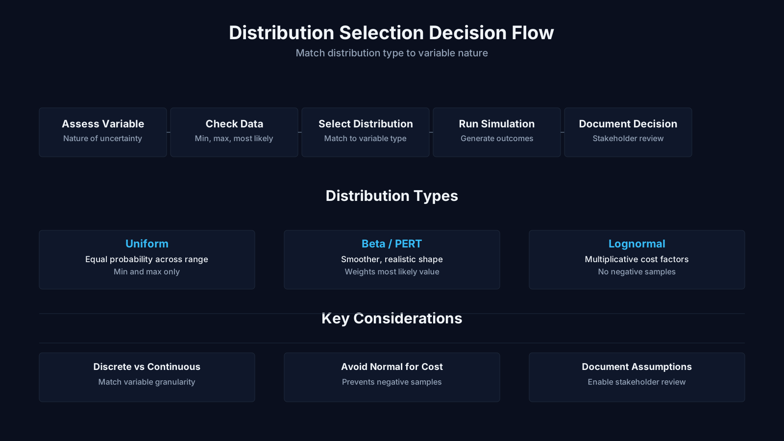
Selecting the right probability distribution is one of the most consequential tasks in quantitative risk analysis. Selecting the right probability distribution for risk models requires matching the shape of the distribution to the nature of the underlying uncertainty, the available data, and the way experts think about the variable. A mechanical default to the normal distribution or the triangular distribution can produce misleading risk outputs even if the simulation software runs perfectly.
The first step is to examine the bounds of the variable. If a cost cannot go below zero and has an upper limit, a bounded distribution like beta or triangular may be appropriate. If the variable has no natural upper bound but is positively skewed, the lognormal distribution may fit better. If the team genuinely has no basis to favor one value over another within a range, the uniform distribution is the honest choice. These distinctions are not about statistical elegance; they are about correctly encoding what the project knows and does not know.
Data availability also drives the selection. With abundant historical data, the analyst can fit distributions using statistical methods. With sparse data, the team often relies on expert three point estimates. In that case, triangular and beta distributions are practical because they align with the familiar optimistic, most likely, and pessimistic values. The risk facilitator should document why each distribution was chosen so that the model can be reviewed and updated later.
Common pitfalls include choosing a distribution because it is the software default, confusing the triangular distribution with the beta distribution, and using the normal distribution for clearly skewed cost data. Another frequent mistake is setting distribution bounds so wide that the model exaggerates uncertainty. Conversely, narrow bounds may clip important tail risk. The right choice emerges from facilitated discussion among technical experts, cost estimators, and risk analysts.
What this means in practice is that distribution selection is a decision, not a formality. The project team should be able to explain in plain language why a particular curve shape reflects reality. If they cannot, the risk model may be hiding assumptions that deserve challenge. A well-documented distribution rationale improves stakeholder confidence and makes the quantitative risk analysis easier to defend during project reviews.
Selecting Common Probability Distributions for Risk Analysis by Shape
The shape of uncertainty often reveals itself in the way experts talk about a variable. If an expert says "it is usually around 15 days but could go as high as 40," that suggests a right-skewed distribution. If another says "any value between 10 and 20 is equally possible," that points to a uniform distribution. If a third says "it is symmetric around 25, sometimes a little less, sometimes a little more," a normal distribution may be reasonable if the bounds are not hard constraints.
Project teams can also test distribution choices by comparing simulation outputs with known historical results. If a model regularly produces outcomes that the team knows are impossible or wildly inconsistent with past projects, the distribution parameters likely need adjustment. This iterative calibration is part of mature quantitative risk analysis, not a sign of failure.
Probability Distributions and the Risk Management Process
Probability distributions do not operate in isolation. They sit inside the broader risk management process, feeding the analysis that informs contingency reserves, schedule buffers, and risk response planning. Quantitative risk analysis process integration is essential because distribution outputs become useful only when they connect to decisions. A Monte Carlo simulation that produces a range of possible project costs is valuable if it leads to a defensible contingency reserve, not merely a chart in a report.
In PMBOK, this activity falls under the Project Risk Management knowledge area, specifically the Perform Quantitative Risk Analysis process. The distributions described earlier are inputs and modeling choices within that process. They support the calculation of expected monetary value, schedule risk, and cost risk at the project or portfolio level. The risk register, project schedule, and cost estimates provide the raw data, while the distributions define the shape of uncertainty around those data points.
PRINCE2 addresses risk through its risk theme, focusing on probability and impact assessment. Quantitative distribution modeling is not as central in PRINCE2 as it is in PMI-style quantitative risk analysis, but the concepts are compatible. A project using PRINCE2 can still apply beta, triangular, or lognormal distributions when deeper numerical analysis is justified. The governance framework does not prohibit robust quantification; it simply often leaves room for proportionality.
Agile environments tend to manage risk through iterative delivery, empirical feedback, and frequent inspection rather than heavy upfront simulation. However, quantitative models still appear in release planning, throughput forecasting, and program-level risk discussions. Flow metrics and Monte Carlo simulation of cycle times use skewed distributions like lognormal to represent the variability of delivery. The same underlying mathematical principles apply, even if the language and cadence differ.
BVOP includes a separate product risk management approach with quantified Loss size units and dynamic filtering. That perspective treats risk as something to be managed through value-oriented filters rather than static probability impact grids alone. A BVOP-informed risk model might still use common probability distributions, but it would tie the risk outputs directly to business value and product decisions, reducing the chance that distribution modeling becomes an academic exercise.
Using Common Probability Distributions for Risk Analysis to Support Decisions
The most effective risk teams connect distribution outputs directly to specific project decisions. If a simulated project cost range indicates that a 15 percent contingency provides only a 60 percent confidence level, the sponsor can decide whether that confidence level is acceptable. If a schedule simulation shows that a particular milestone has a high probability of slipping beyond a contractual date, the team can plan a risk response. Distribution outputs without a decision link often remain unused.
Risk distributions also support trade-off analysis. A project manager can compare the probability of finishing within a target budget under different response strategies. By adjusting the distribution parameters to reflect a proposed risk response, the team can estimate whether the response meaningfully shifts the risk profile. This turns quantitative risk analysis from a reporting exercise into an active management tool.
Key Takeaways on Distribution Integration
- Distributions drive risk decisions
- Probability distributions inform contingency reserves, schedule buffers, and risk response strategies, translating uncertainty into actionable inputs for the broader risk management process.
- Value requires decision linkage
- Distribution outputs create value only when they support concrete decisions, such as justifying a defensible contingency reserve that guides budget allocation, instead of existing as a standalone chart in a report.
- PMBOK process placement
- Within the PMBOK framework, this activity belongs to the Perform Quantitative Risk Analysis process in the Project Risk Management knowledge area, where distributions function as both modeling inputs and parameters that shape the analysis.
- Adaptable across frameworks
- PRINCE2 supports scaled use of distributions based on project complexity, Agile favors iterative feedback cycles over heavy upfront simulation, and BVOP links distribution outputs directly to business value and product decisions.